Motivational Image
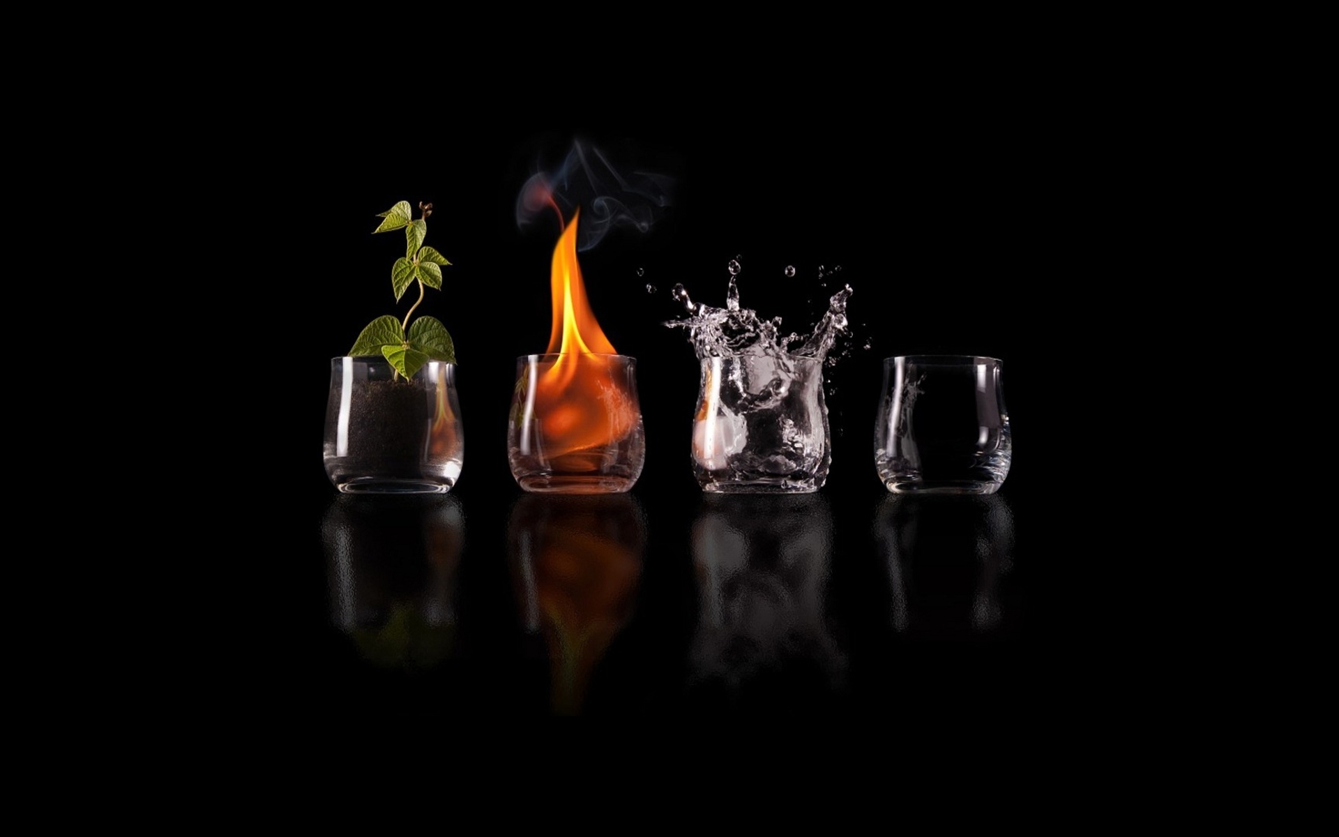
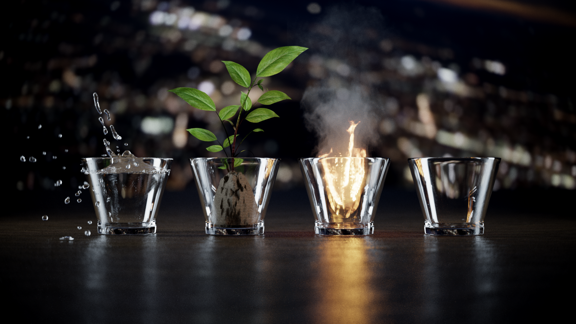
The motivational image depicts four natural elements: earth, fire, water and air. I did not intend to reproduce the image closely, but I liked the main idea and composition. The image shows a few interesting phenomena for rendering, e.g. glossy reflections, heterogeneous media and light emission from volumes.
Motivational Image
Third Party Libraries
In addition to the libraries already used by Nori from the beginning, the following libraries have been added:
- cxxopts - for parsing command line arguments
- lodepng - for saving PNG images
- openvdb - for OpenVDB volume grid support
- sobol - for sobol sequences used in the sobol sampler
Basic Features
The following features I have already implemented as part of the renderer I created for the 2014 Image Synthesis class. They are not graded so there is no in-depth description/verification of their implementation.
- Thin Lens Camera
- Bump Mapping
- Blend BSDF - blends between two BSDFs based on a mix texture
- Conductor BSDF - using complex IOR
- Rough Conductor BSDF - using microfacet model and complex IOR based on [6]
- Rough Diffuse BSDF - using qualitative Oren-Nayer model based on [7]
- Transparent/Forwarding BSDF
- Sobol Sampler using Sobol implementation from [8]
- Bitmap Texture
- Scale Texture
- Environment Map Emitter with Importance Sampling based on [5]
- Homogeneous Media
Disney BRDF
include/nori/bsdf.hsrc/bsdfs/disney.cpp
Surface appearance is very important for generating realistic images. Having implemented a whole list of different BSDFs in the past, I wanted to implement something more flexible this time, even if it is not fully physically correct. I decided to implement Disney's Principled BSDF, which is thoroughly described in [1]. Additional information is available in [2] and [3]. This BSDF is physically based but not completely physically correct (e.g. not always energy conserving). It was designed with the following principles in mind:
- Intuitive rather than physical parameters should be used.
- There should be as few parameters as possible.
- Parameters should be zero to one over their plausible range.
- Parameters should be allowed to be pushed beyond their plausible range where it makes sense.
- All combinations of parameters should be as robust and plausible as possible.
The BRDF is parametrized by a single color value and a set of scalar values in the range \([0..1]\). The effect of these parameters is shown in the following image:
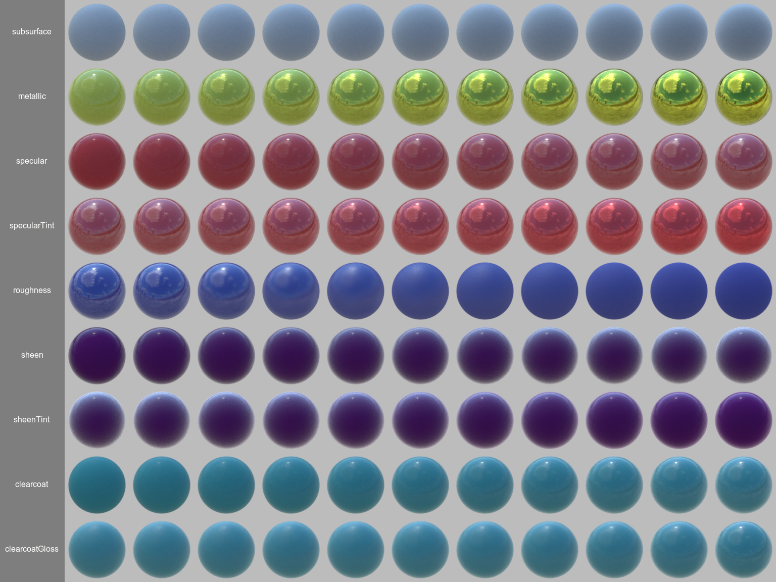
Visualization of the Disney BRDF parameters (rendered in Nori)
Verification
Verifying the BSDF is not an easy task, as there is no reference implementation to compare against. In the following sections I show qualitative comparisons against BSDFs in Mitsuba as well as point out some of the expected behavior of the BSDF.
Variables and Terms
\( \theta_i \) Incident angle
\( \theta_o \) Exitant angle
\( \theta_h \) Half angle
\( lerp(t,a,b) = (1-t)a + tb \)
Fresnel Terms
Instead of using the full fresnel equations, the Disney BRDF uses Schlick's approximation defined as follows:
\[ F(\theta) = (1 - \cos{\theta})^5 \]Diffuse Model
Instead of relying on the default Lambert or Oren-Nayer diffuse reflection models, the Disney BRDF uses an empirical model, which reduces the diffuse reflectance by 0.5 at grazing angles for smooth surfaces and increases the reflectance by up to 2.5 for rough surfaces. The diffuse reflection model is defined as follows:
\[ f_d(\theta_i,\theta_o) = \frac{baseColor}{\pi} (1 + (F_{D90} - 1) F(\theta_i)) (1 + (F_{D90} - 1) F(\theta_o)) \] \[ F_{D90} = 0.5 + \cos{\theta_h}^2 roughness \]
The following clearly shows the decreased/increased reflectance at grazing angles compared to the Lambert model:
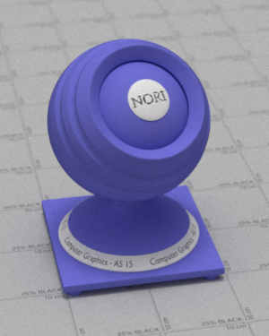
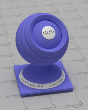
\[roughness = 0.0\]

\[roughness = 0.5\]
\[roughness = 1.0\]
Subsurface Model
To model subsurface scattering the Disney BRDF blends between the diffuse model and a Hanrahan-Krueger inspired model. This subsurface scattering model is a very crude approximation and only works for materials with very short mean free paths.

Subsurface Model
Specular / Clearcoat Model
The specular lobes use a standard microfacet model defined by:
\[ f_s(\theta_i, \theta_o) = \frac{D(\theta_h)F(\theta_i)G(\theta_i,\theta_o)}{4\cos\theta_i\cos\theta_o} \]where \(D\) is the normal distribution, \(F\) is the fresnel term and \(G\) the shadowing term For the normal distribution, the Generalized-Trowbridge-Reitz (GTR) is used:
\[ D_{GTR}(\theta_h) = \frac{c}{(\alpha^2 \cos^2\theta_h + \sin^2\theta_h)^\gamma} \]where \(c\) is a normalization constant and \(\alpha\) is the roughness value. Two specular lobes are used, the main specular lobe using \(\gamma = 2\) and the clearcoat lobe using \(\gamma = 1\). Instead of specifying the IOR explicitly, the BRDF uses the \(specular\) parameter, which maps to a range of \([0..0.8]\), that corresponds to IOR values of \([1..1.8]\), where the middle value corresponds to an IOR of \(1.5\) (polyurethane). For the clearcoat lobe, a fix IOR of \(1.5\) is used, and the strength is based on the \(clearcoat\) parameter that is scaled to a range of \([0..0.25]\). The roughness value of the specular lobe is defined as \(\alpha = roughness^2\), whereas the roughness value of the clearcoat lobe is defined as \(\alpha = lerp(clearcoatGloss, 0.2, 0.001)\).
For the shadowing term \(G\) the standard smith shadowing term is used. However, Disney uses some strange tweaks (adjusting roughness value) to the shadowing term, which is motivated from artists that complained about specular being too hot at grazing angles. When comparing the specular component against Mitsuba renderings, this darkening at grazing angles is clearly visible and I personally don't like it too much.

\[roughness = 0.0\]
\[roughness = 0.2\]


\[roughness = 0.4\]
\[roughness = 0.0\]
\[roughness = 0.2\]
\[roughness = 0.4\]
Sheen Model
Too add in sheen, typically observed in cloth materials, the following simple term is used:
\[ f_{sheen} = F(\theta_h) \cdot sheen \cdot lerp(sheenTint, 1, baseColor) \]
Importance Sampling
For efficient sampling of the Disney BRDF, I have implemented an importance sampling scheme based on the following three samplable distributions:
- Cosine weighted hemisphere
- GTR1 normal distribution
- GTR2 normal distribution
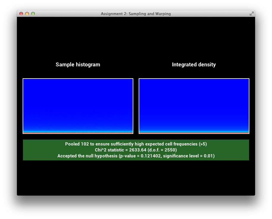
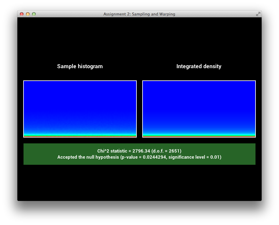
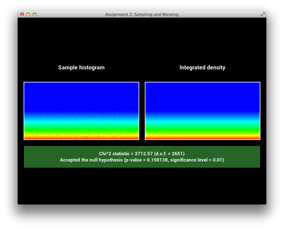
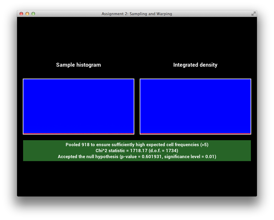
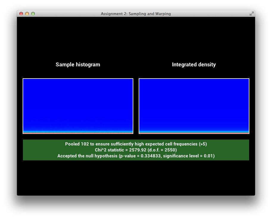
First, I have verified that sampling the GTR1 and GTR2 distributions works correctly by testing them in the provided framework.
GTR1 Sampling Verification

\[\alpha = 0.05\]
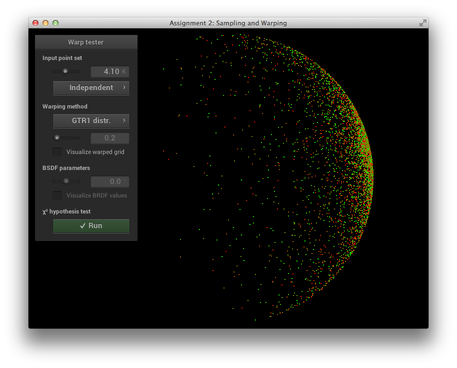
\[\alpha = 0.2\]
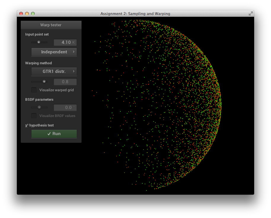
\[\alpha = 0.8\]
\[\alpha = 0.05\]
\[\alpha = 0.2\]
\[\alpha = 0.8\]
GTR2 Sampling Verification
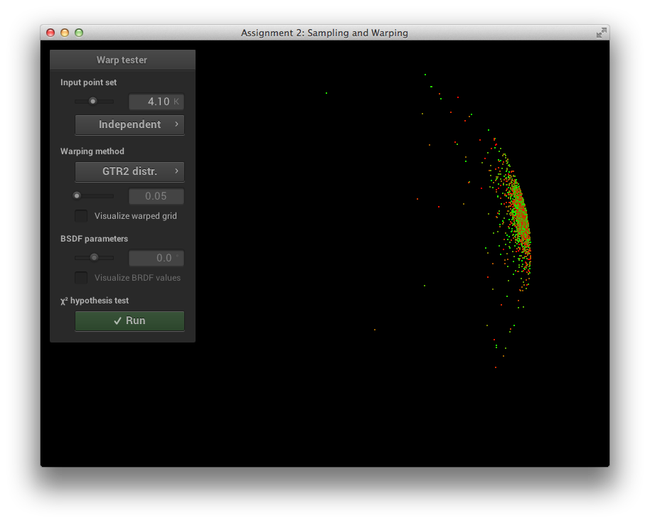
\[\alpha = 0.05\]
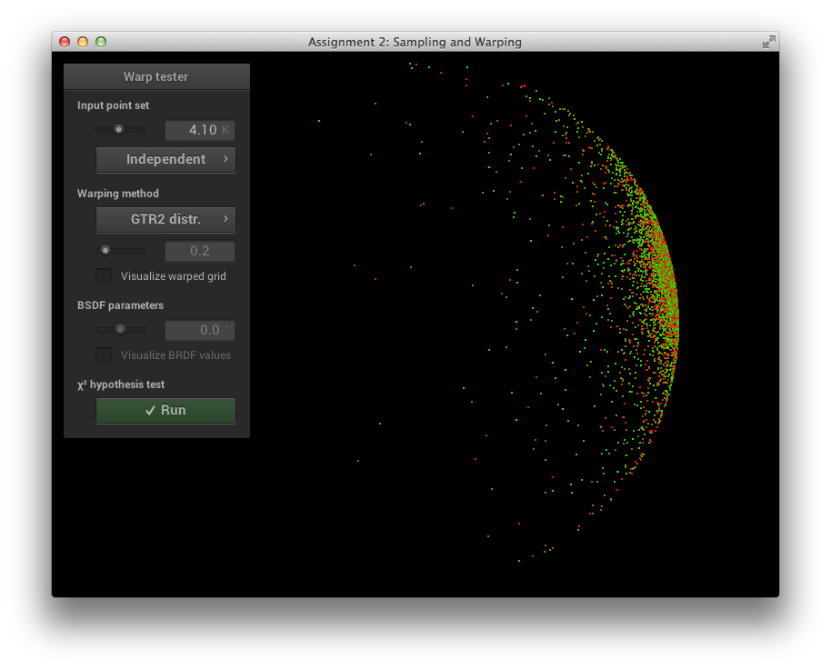
\[\alpha = 0.2\]

\[\alpha = 0.8\]
\[\alpha = 0.05\]
\[\alpha = 0.2\]

\[\alpha = 0.8\]
For sampling the BRDF, I first use russian roulette to decide between sampling the diffuse lobe or the specular lobes with the following ratio:
\[ ratio_{diffuse} = \frac{1 - metallic}{2} \]e.g. for non-metallic materials, half of the samples are sampled with cosine weighted hemisphere sampling, the other half with specular sampling described below. For metallic materials, all samples are sampled using specular sampling.
The specular samples are divided into sampling the GTR2 (specular lobe) and GTR1 (clearcoat lobe) distribution with the following ratio:
\[ ratio_{GTR2} = \frac{1}{1 + clearcoat} \]e.g. for materials with no clearcoat, samples are only sampled using the GTR2 distribution, for materials with 100% clearcoat, half the samples are directed to either of the distributions.
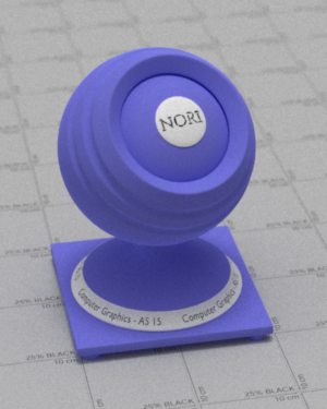
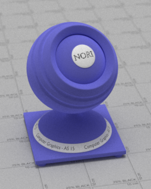
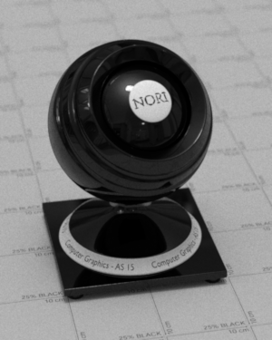
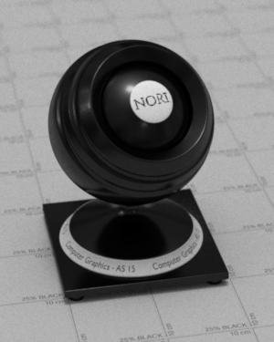
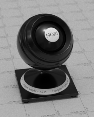
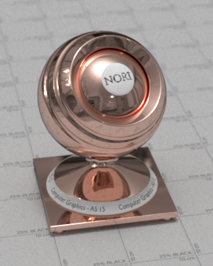
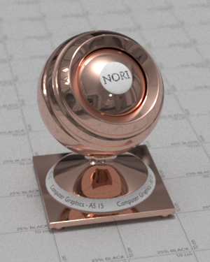
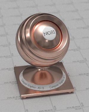
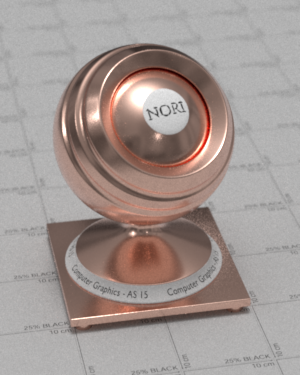
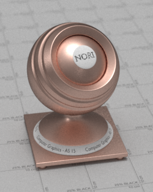
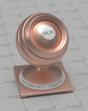
Finally, the following shows a few materials that I rendered using the Disney BRDF:
Materials made using the Disney BRDF
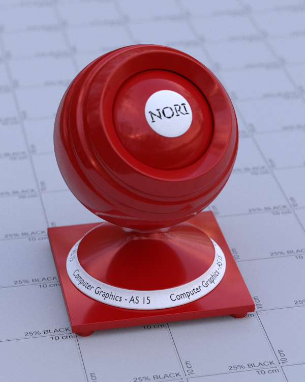
Plastic
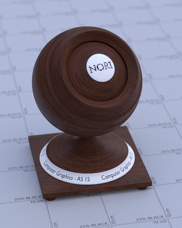
Wood
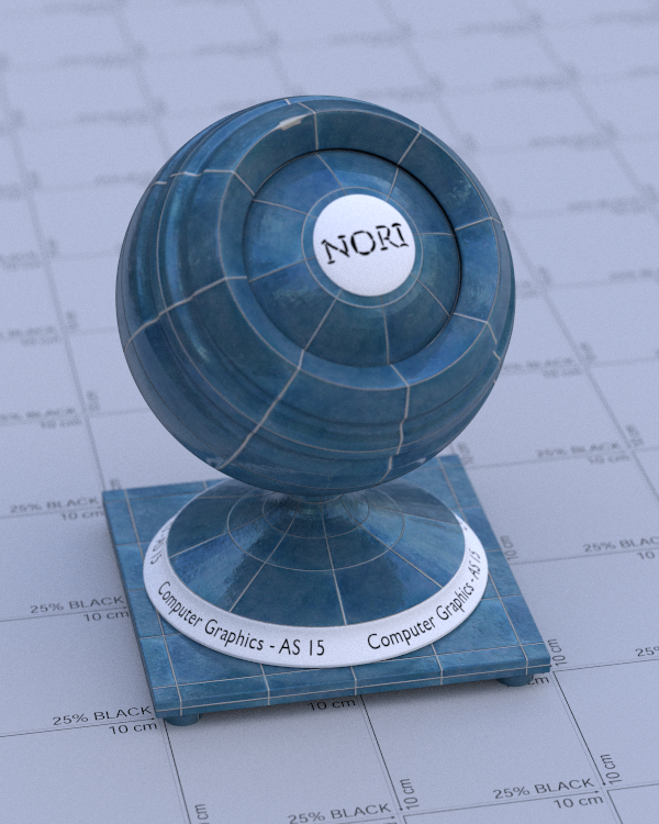
Ceramic Tiles

Concrete
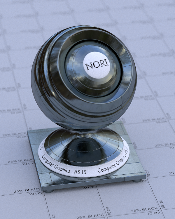
Metal Panels
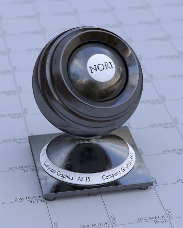
Scratched Metal
Realistic Camera
src/cameras/realistic.hsrc/cameras/realistic.cppsrc/lenstest.cpp
In order to create photo-realistic images, a good approximation of the camera lens system is essential. The simplest lens approximation is the pinhole camera, which essentially simulates a lens with infinitely small aperture. Most photographs are taken with larger apertures however, because it lets more light hit the film/sensor, generating less noisy photographs. Also, larger apertures lead to a more shallow depth of field, which allows to separate a subject from the background and create a better sense of depth in the photograph. To simulate the effect of a larger aperture, one can use the thin lens approximation [12]. This allows for better realism but it is still a rather crude approximation when compared to a real camera lens system. Many of the artifacts that happen in a real lens such as cat's eye, vignetting, non-planar focus region and others have to be faked when using the thin lens model. This is why I have decided to implement a more realistic camera model based on [4]. The basic idea is to shoot rays through a bunch of spherical lens elements, essentially simulating what happens in a real camera lens system. For debugging and testing purposes I have also implemented a lens testing application, which was used to generate all the following screen shots.
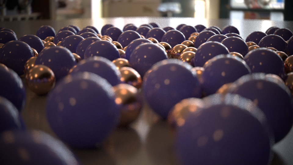
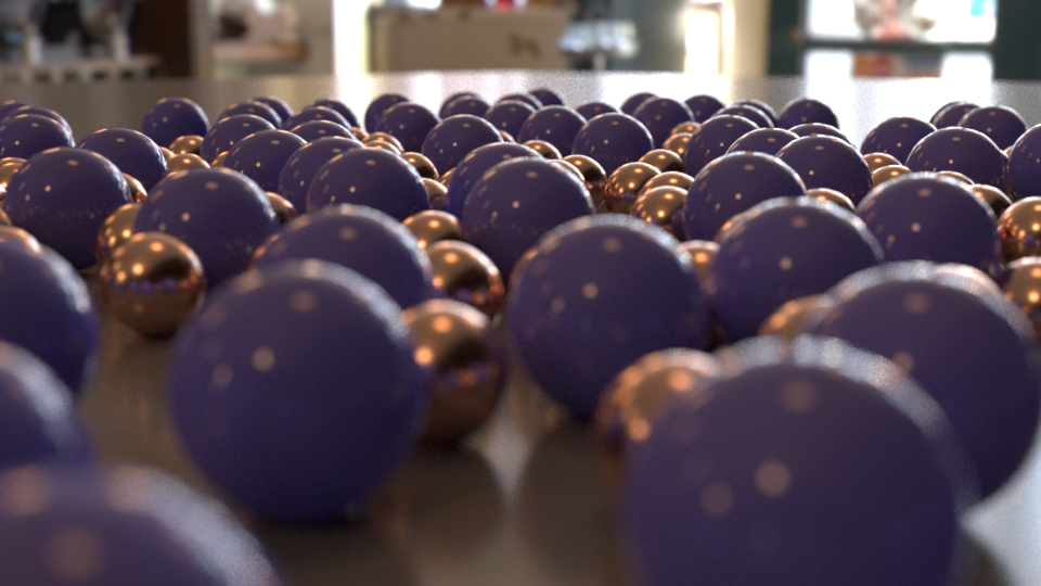
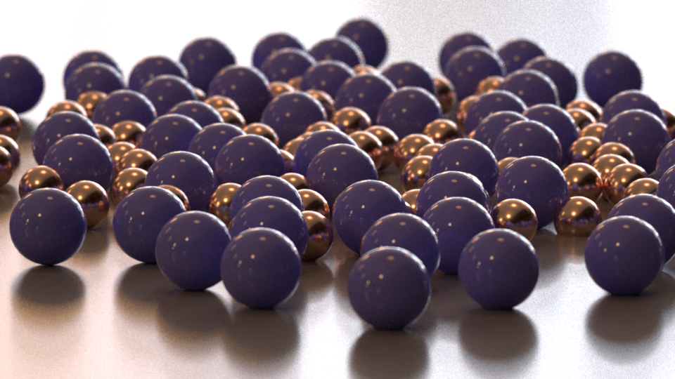
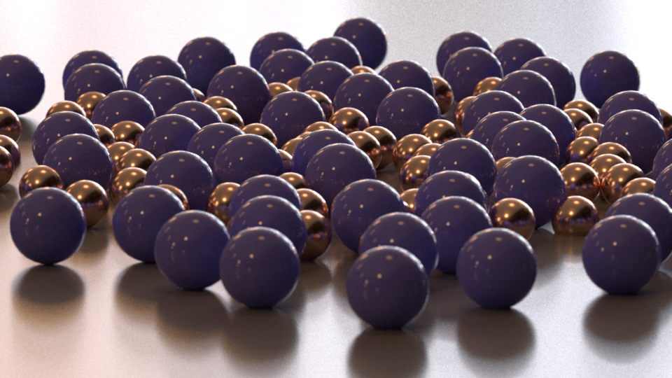
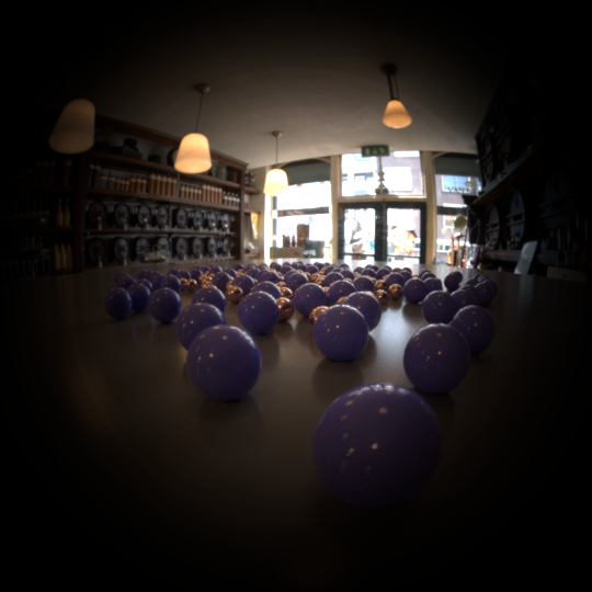
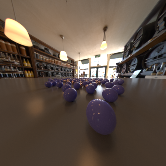
The following images show a 50mm lens with different aperture values. With smaller apertures, less light hits the sensor and the passing light paths get more and more parallel, resulting in a larger focus region.
Aperture
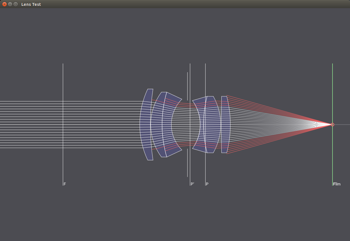
f/2

f/4
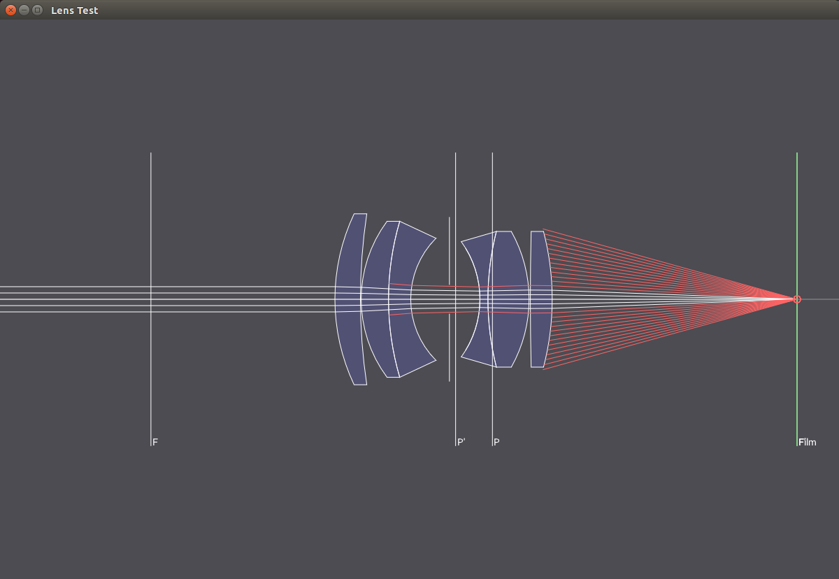
f/8
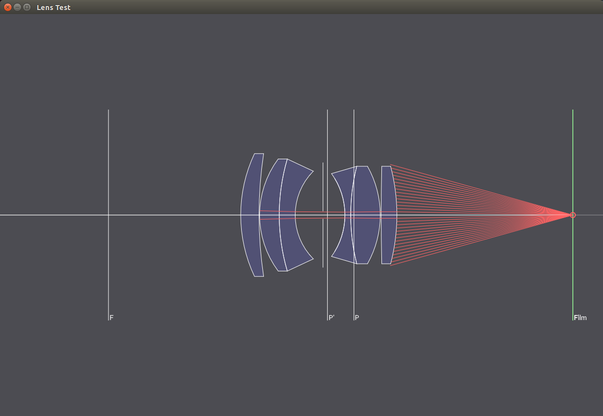
f/22
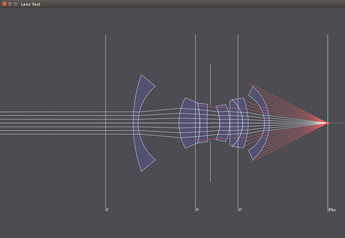
The following images show the lens elements used in different photographic lens systems.
Lenses
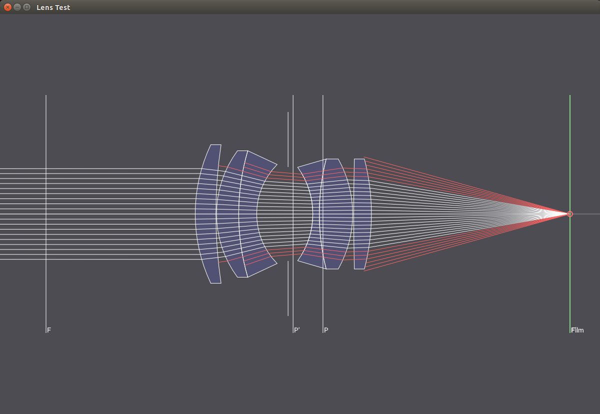
Double Gauss 50mm

Fisheye 10mm

Telephoto 250mm
Wide 22mm
In the next images, a 50mm lens is focused at different distances, which is accomplished by moving the lens relative to the film plane.
Focusing
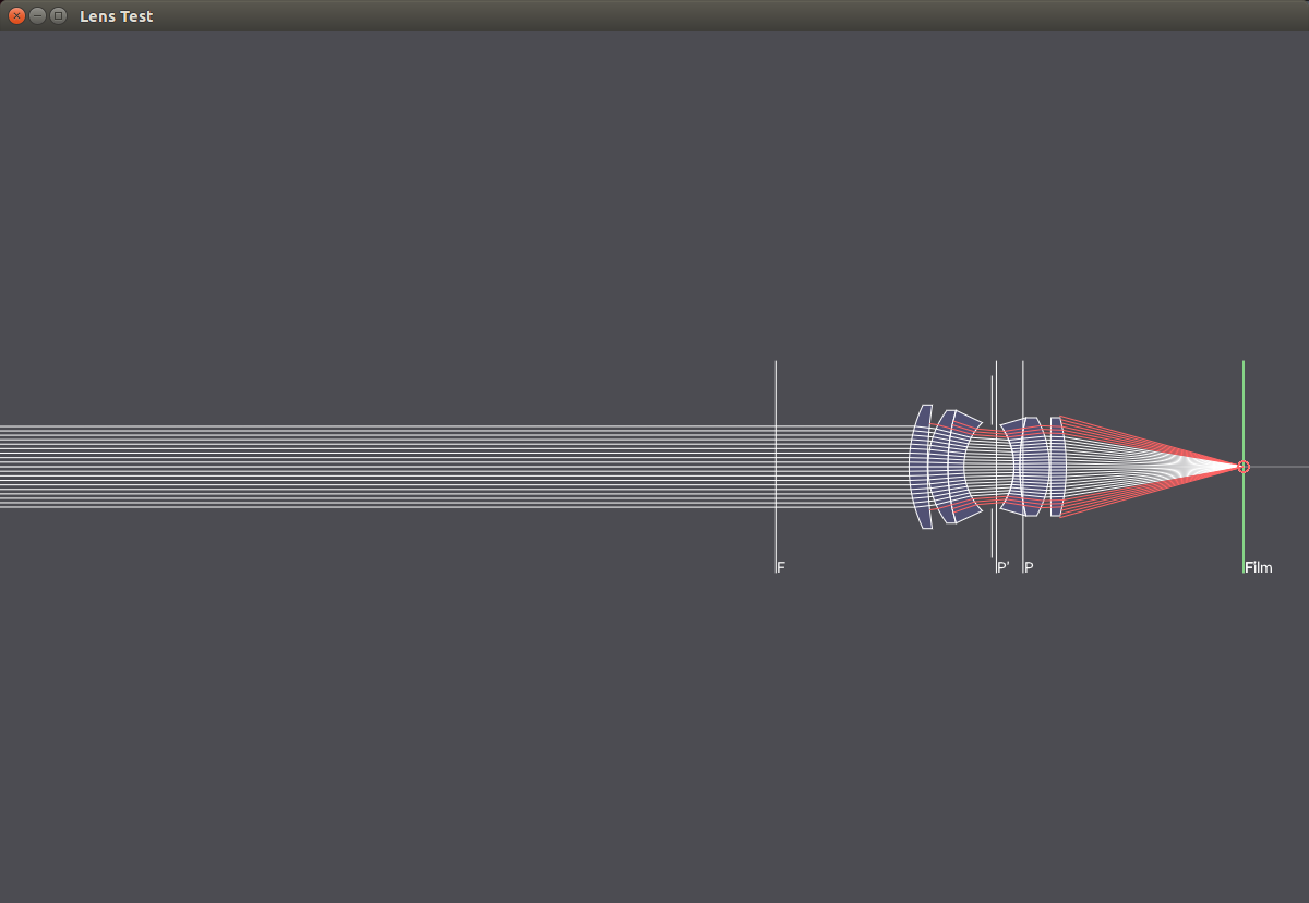
Focused to Infinity
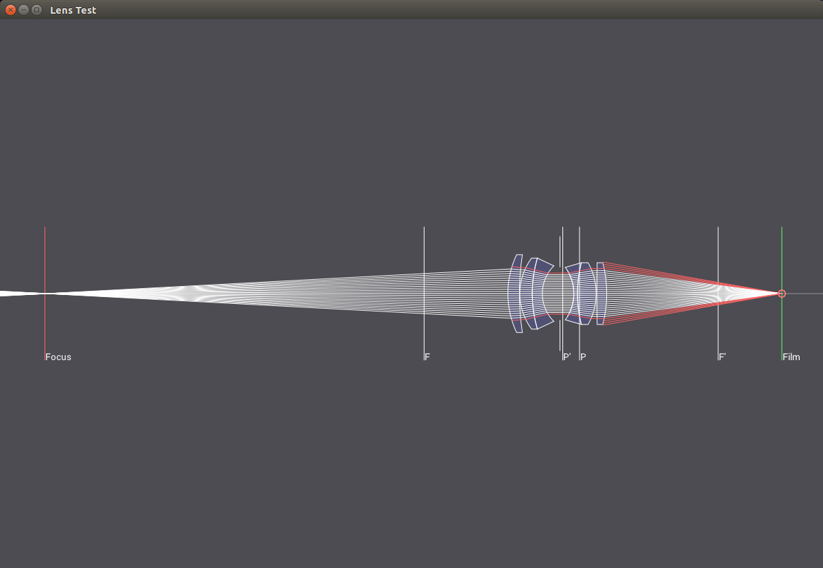
Focused to 0.1m
Finally, the following images show comparisons between images rendered with the thin lens and the realistic lens model. It clearly shows some of the benefits of simulating a realistic lens model such as vignetting, cat's eye bokeh, barrel distortion, non-planar focus plane and others. Some of these effects might be considered artifacts and are usually tried to be minimized in modern lens designs, however, in my opinion they do contribute a lot towards the realism of the generated images.
Double Gauss 50mm
Telephoto 250mm
Fisheye 10mm

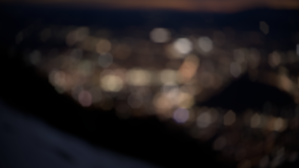
Bokeh
Heterogeneous Media
include/nori/medium.hinclude/nori/phasefunction.hinclude/nori/piecewiselinear.hinclude/nori/volume.hsrc/integrators/volpath.cppsrc/mediums/heterogeneous.cppsrc/phasefunctions/hg.cppsrc/phasefunctions/isotropic.cppsrc/volumes/const.cppsrc/volumes/grid.cppsrc/volumes/grid.hsrc/volumes/vdb.cppsrc/volumes/vdbutils.h
In order to render the fire and smoke effect for my final image, I needed an implementation for rendering heterogeneous media. In a first step, I implemented rendering of simple homogeneous media, so I had a reference to compare my implementation of heterogeneous media against. I also implemented two versions of volumetric path tracers. The first one, volpath_naive, is based on the path_mats integrator, but extends it with sampling distances in media and sampling the phase function. The resulting integrator is extremely inefficient, but due to its simplicity, a good reference to compare against. The second more complex integrator, volpath_mis, is based on the path_mis integrator and extents it with sampling distances in media and sampling the phase function. It uses multiple importance sampling and combines sampling direct lighting as well as sampling the phase function, similarly to sampling direct lighting and the BSDF. This leads to a fairly efficient unidirectional volumetric path tracer.
Heterogeneous media are typically represented by voxel grids. In order to do some comparisons with Mitsuba, I first implemented a voxel grid that can read Mitsuba's voxel data format. In addition, I also implemented a voxel grid based on OpenVDB, to allow for more elaborate voxel data authoring using Houdini. To sample distances in the heterogeneous medium, I took a slightly different approach than the usual inversion of the transmittance. Instead, based on ideas from [11], I raymarch through the volume, create a transmittance function, and then create a PDF based on the transmittance multiplied with the scattering coefficient. This PDF can then be used to sample scattering distances inside the medium. The transmittance function is cached in order to be reused when accounting for volume emission (see next section).
The following two comparisons show the correct rendering of heterogeneous media. The reference images are rendered using a sphere with a forwarding BSDF that contains a homogeneous medium. The same sphere is then created using a voxel grid (hence the visible voxelization artifacts) and rendered as heterogeneous media. Other than some minor bias (due to the raymarching), both images should be equal, which is clearly the case. As an additional validation, the last comparison shows a heterogeneous medium rendered in both Nori and Mitsuba.
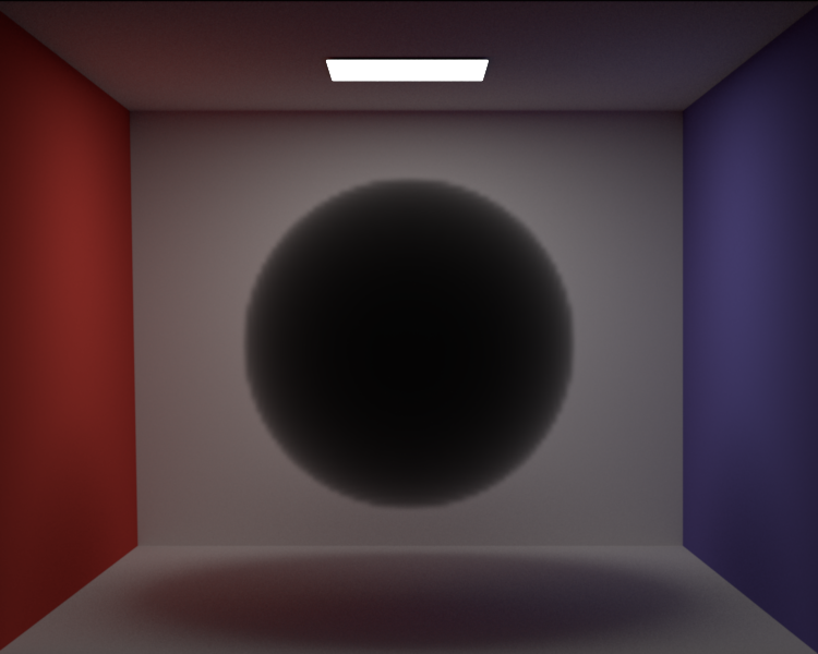
Comparison between homogeneous and heterogeneous media without scattering
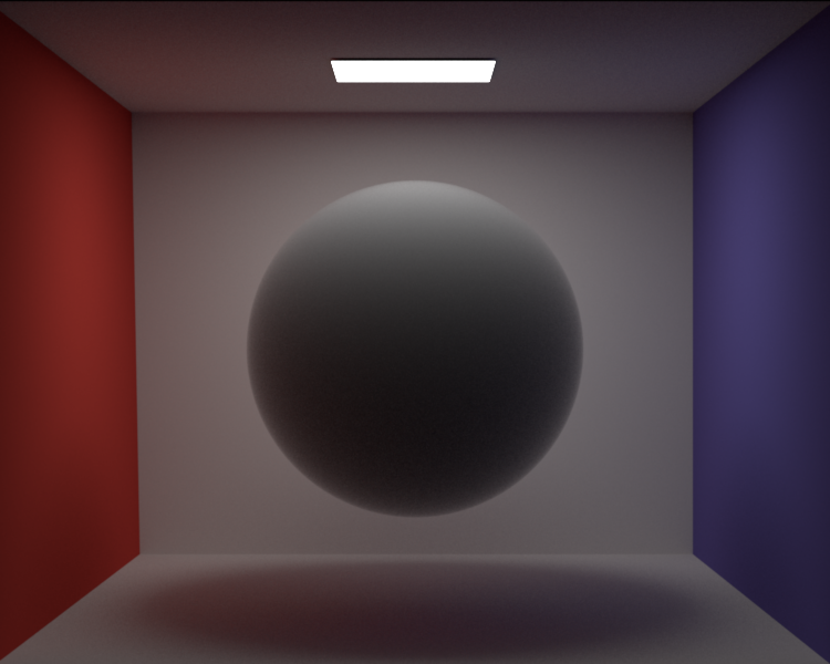
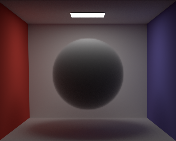
Comparison between homogeneous and heterogeneous media with scattering

Comparison between Nori and Mitsuba
Volume Emission
include/nori/cie.hinclude/nori/spectrum.hsrc/emitters/medium.cppsrc/mediums/heterogeneous.cppsrc/volumes/fire.cppsrc/cie.cpp
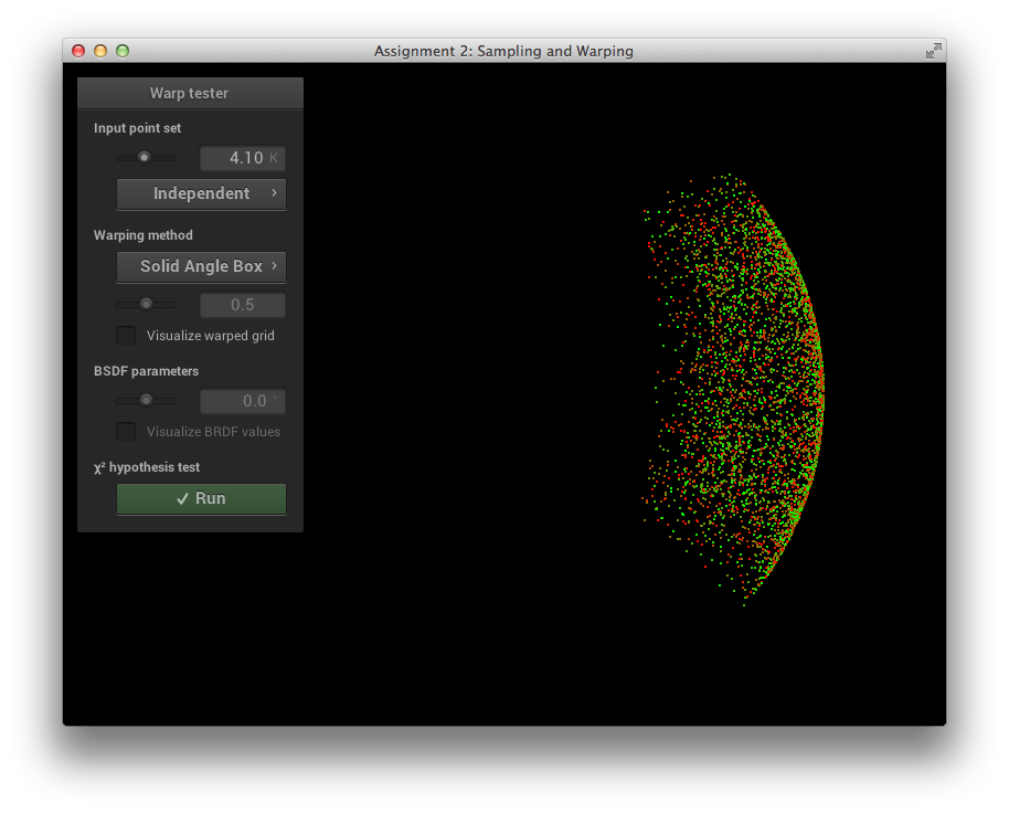
In addition to absorption and scattering in heterogeneous media, I also needed to implement emission from heterogeneous media to allow for the fire effect of the final image. For more efficient sampling of emission from volumes, I added support for volumetric emitters, such that direct lighting can be sampled with respect to solid angle, similarly to surface based emitters. Unfortunately this is a little more involved than for surface based emitters, because volume emitters are not opaque. Computing the probability for choosing a direction for direct lighting thus needs to account multiple emitters, not just the nearest to the shading location. In order to sample a direction towards emissive volumes, I use the following simple approach, extended from ideas presented in [10]: First, a bounding box around the emissive part is computed. Next, a position is sampled within the bounding box using uniform sampling. This position determines the direction from the shading location. To compute the PDF, we simply compute the integral of the probabilities of choosing all points inside the bounding box that lie on the ray from the shading location to the sampled position inside the bounding box. I planned to extend this idea from a single bounding box per emitter into a emission grid per emitter, each voxel would then be weighted according to the total emission within that voxel, which should decrease variance considerably. Due to time constraints I was not able to implement this idea however. The sampling of a box with respect to solid angle is verified in the following test:
Box Sampling Verification

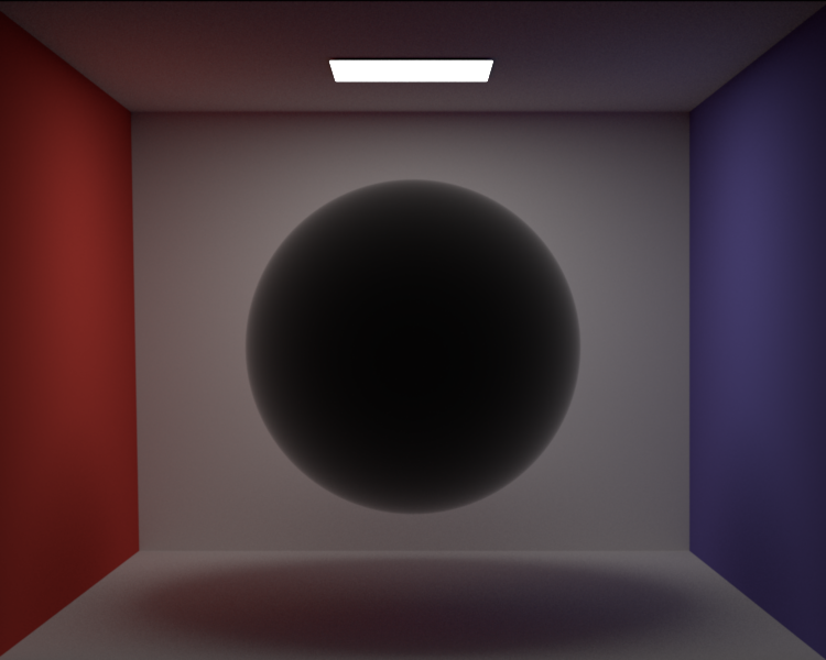
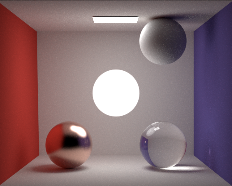
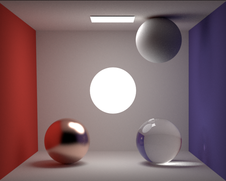
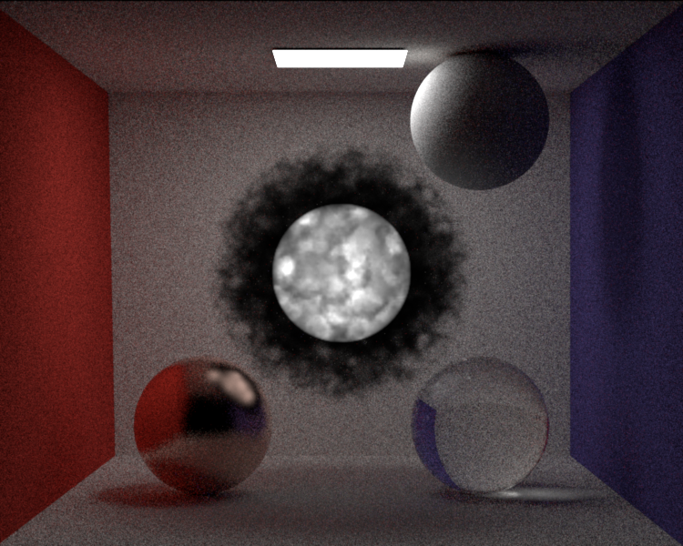
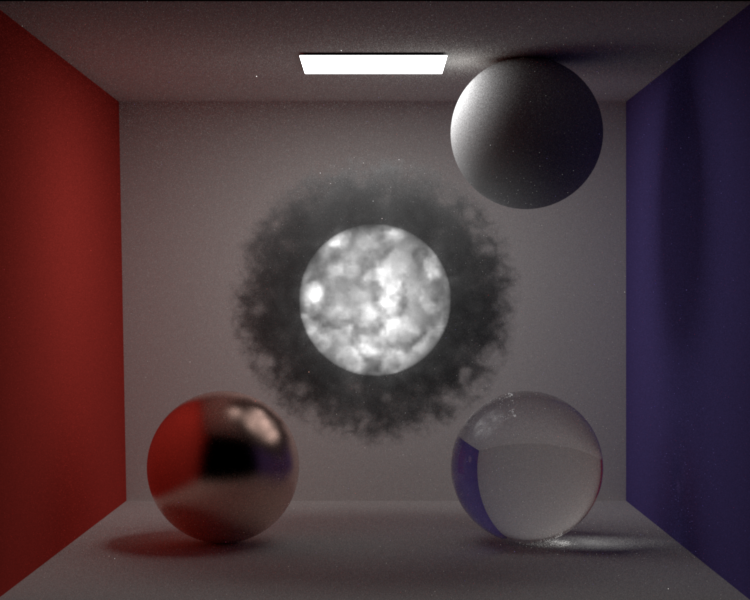
To test volume emission, I set up a scene containing an emissive volumetric sphere in the middle and four spheres around, each with a different BSDFs (rough conductor, dielectric, diffuse and forwarding). Each image was rendered once with the volpath_naive integrator using 512spp, and once with the volpath_mis integrator using 256spp. Render times are roughly equal, but usually the volpath_mis took a little longer. The first comparison shows emission only, with no absorption or scattering. As a comparison, the same scene was also rendered with a surface based emitter, which however does not lead to the exact same results, as the diffuse surface based emitter emits the same radiance in all directions, whereas the volume based emitter emits less radiance with grazing angles (this is clearly visible in the reflections and caustics). The second comparison adds an absorption only heterogeneous medium. The last comparison also adds scattering. The comparisons clearly show the importance of MIS for rendering (emissive) volumes.
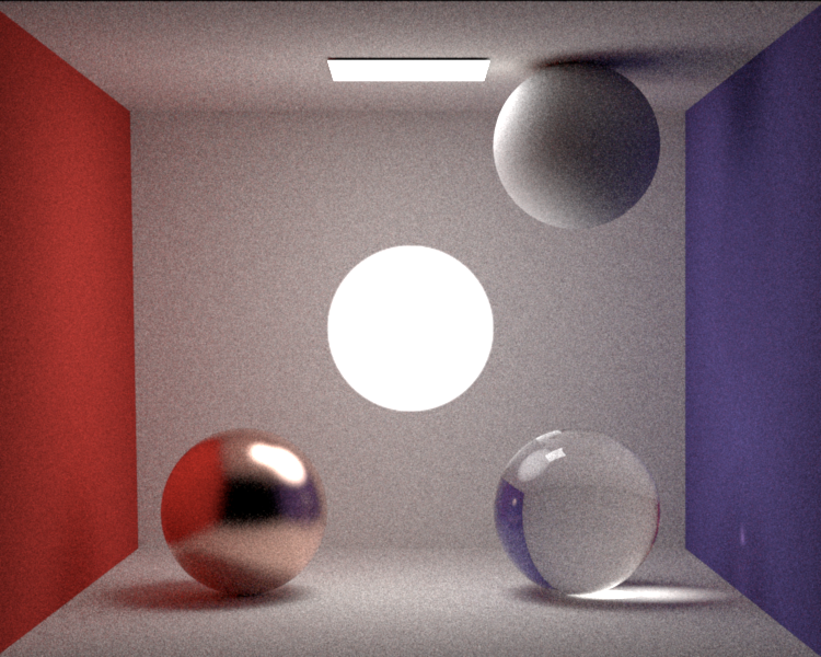
Emissive sphere volume

Emissive sphere volume surrounded in heterogeneous medium without scattering

Emissive sphere volume surrounded in heterogeneous medium with scattering
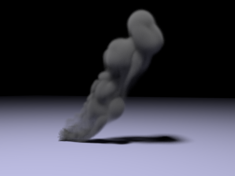
With basic volume emission in place, I needed a way to render flames/fire. Instead of manually coloring the emission volume, I used ideas presented in [9] (chapter 4.5 in the Volume Rendering at Sony Pictures Imageworks part) to derive believable emission from a temperature grid. The results can be seen below:
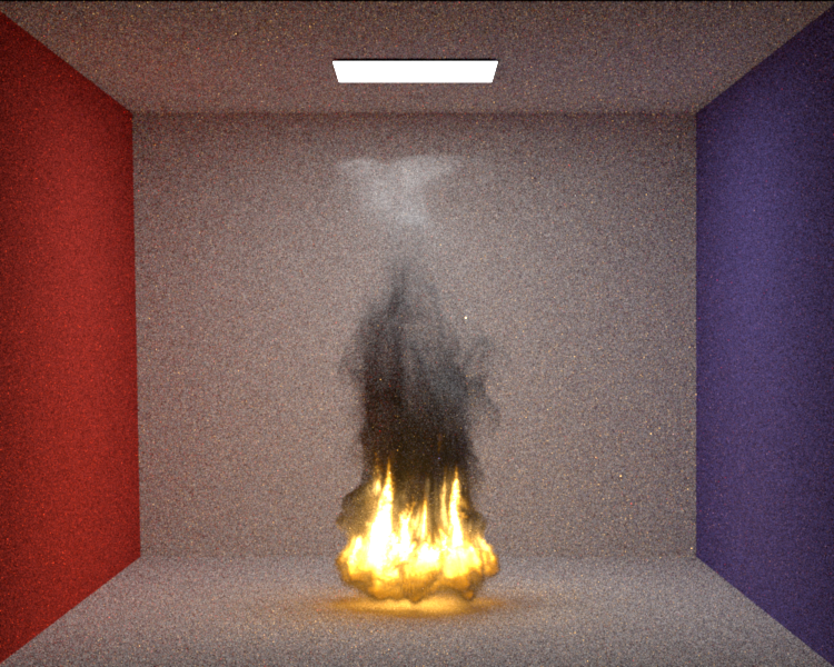
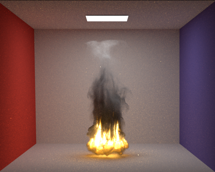
Fire using heterogeneous medium and blackbody emission (using fire.vdb from openvdb.org)
Adaptive Sampling
src/render.cpp
Rendering an image with a Monte Carlo Path Tracer that uses the same number of samples for each pixel is not efficient. This is due to the fact that in complex scenes some areas of the image might converge considerably faster than others. For example, areas with specular reflections may require many more samples to converge in comparison to areas with just diffuse surfaces. To help render my final image, I decided to implement a very simple adaptive sampling method based on [13]. I followed the method described in the paper pretty closely and extended it as follows:
- use gamma correction and color clamping before computing the error metric
- use minimum block size of 8x8 pixels and only allowing regions to be multiples of 8x8 pixels
- progressive rendering by restarting the method with a smaller threshold every time convergence is reached
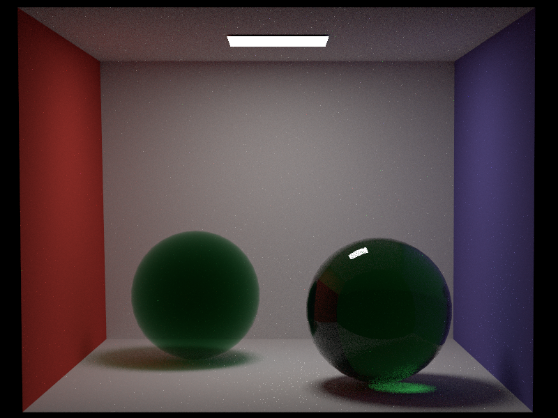
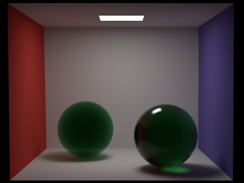
The following comparisons show equal time renderings with and without adaptive sampling. Each iteration uses an error threshold half of the previous iteration. To better highlight the differences, the contrast of the images has been enhanced. The comparisons clearly show how the adaptive sampling method is able to render images with more uniform noise across the image, which is mostly visible in the caustic and the reflections of the sphere on the right. The last comparison shows the sampling distribution when using adaptive sampling, clearly indicating the focus on the regions that converge less quickly.


After 1.2 minutes (error threshold 0.004)


After 4 minutes (error threshold 0.002)

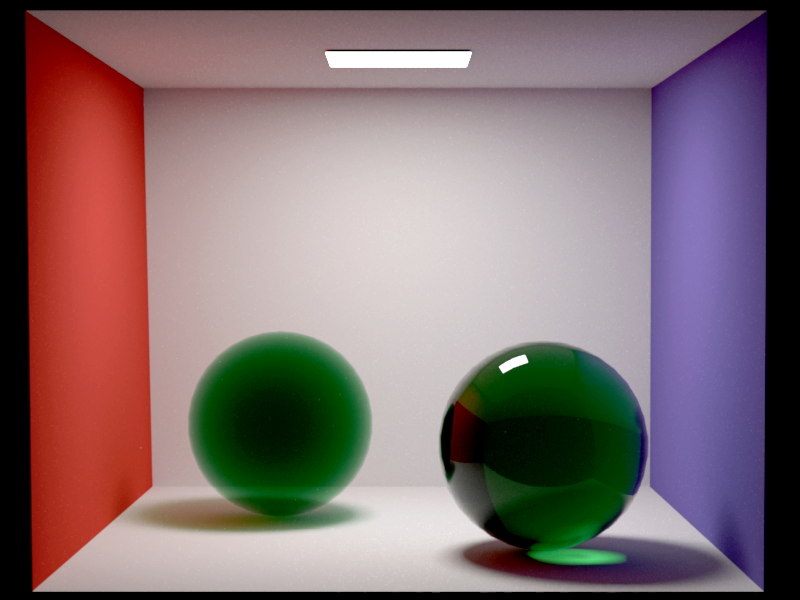
After 11.6 minutes (error threshold 0.001)
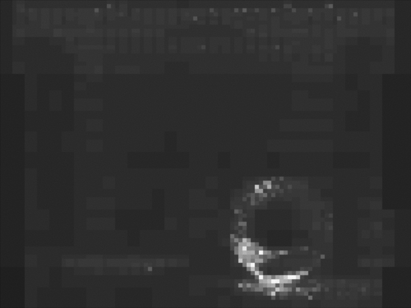
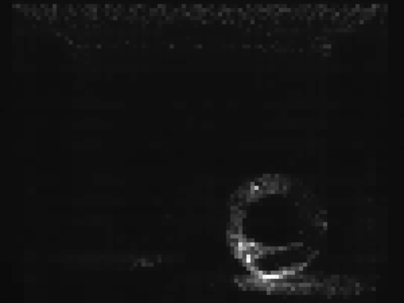
Sampling distribution when using adaptive sampling
Denoising
include/nori/imagebuffer.hinclude/nori/rendertarget.hsrc/imagebuffer.cppsrc/rendertarget.cpp
To further decrease the noise in the final image, I decided to implement a simple denoiser based on [14] and some own ideas. First, I extended the renderer to output some extra data, namely a variance buffer of the rendered color buffer as well as a few additional feature buffers, each with its own variance buffer. The additional features buffers consist of the albedo, normal and depth values. To simplify the generation of the render buffers, I removed the reconstruction filters and just used a simple box filter, which simplifies computation of the variance. The following shows an example of the additional outputs.
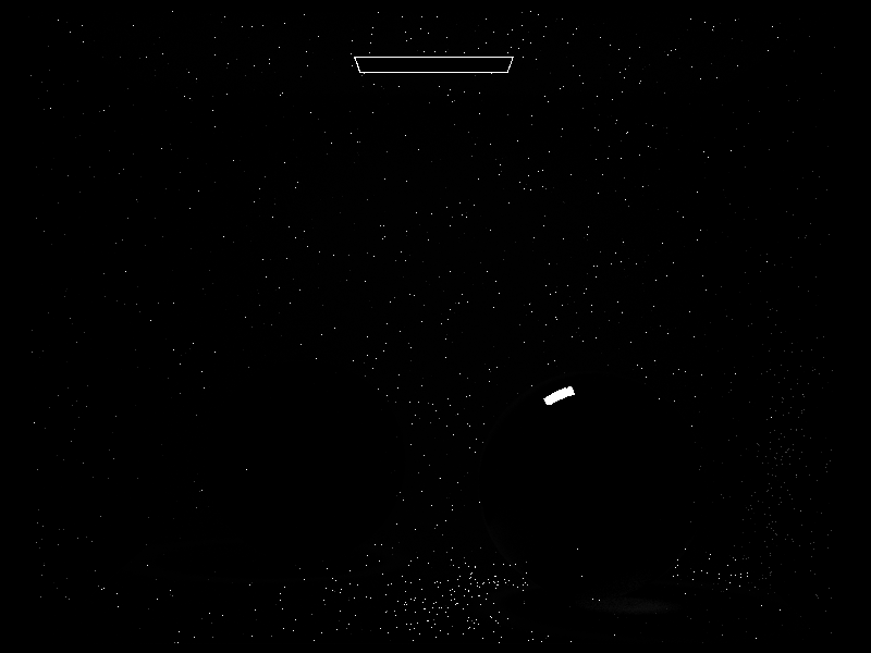
Color Buffer
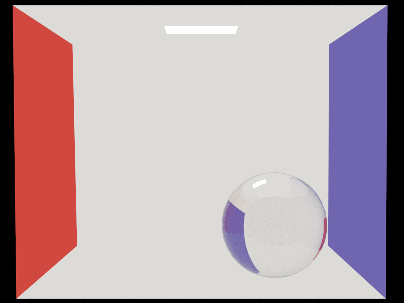
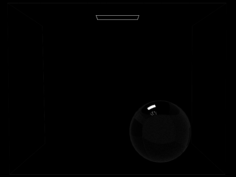
Albedo Buffer
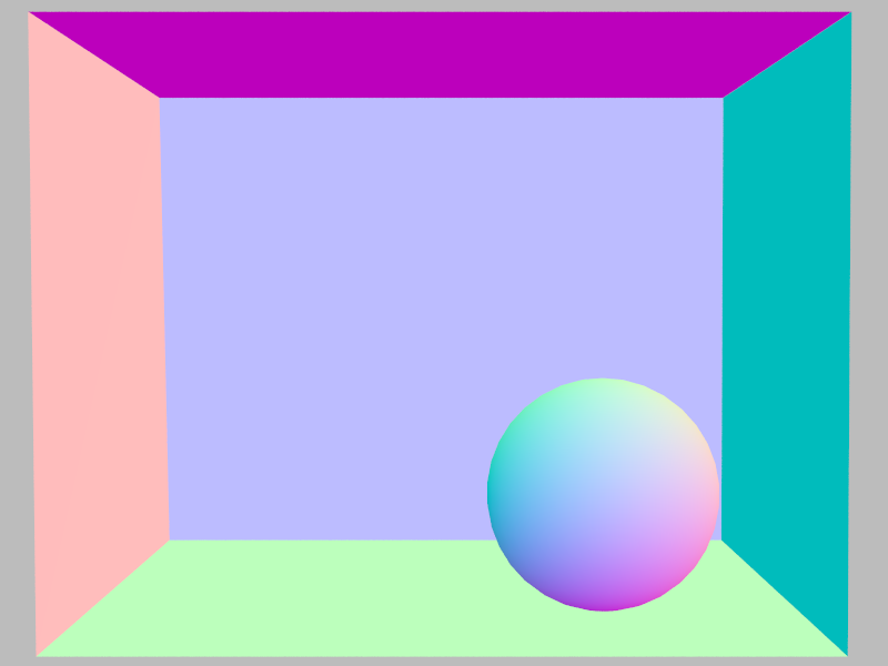
Normal Buffer
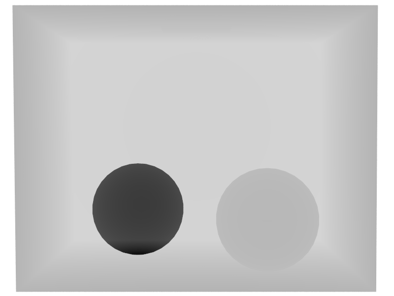
Depth Buffer
In a first step, the denoiser removes fireflies by using a simple heuristic. If a pixel with high variance is only surrounded by pixels with much lower variance, it is marked as a firefly and replaced by taking the average of the surrounding pixels. By default a ratio of 100 is used to detect pixels with high variance. The following shows a before and after comparison.

Firefly filter (removing around 1000 fireflies)
Following the firefly removal, the denoiser uses the NL-means filtering approach described in [14]. While NL-means filtering works relatively well on simple scenes, I didn't used it for my final image. I wasen't able to get the results I was hoping for and the residual noise after removing fireflies was actually more pleasant then the denoised image.
NL-means filter
I also implemented image processing and tonemapping functionality into the denoiser, in order to avoid using any external software for producing the final image (other than scene authoring). I added some basic image processing such as exposure, saturation, color temperature adjustments and an additional tonemapper based on an analytic light response curve for Kodak film based on [15].
Scene Modelling
To create the scene for the final image, I used Blender to model the glasses, the simple scene geometry as well as using the fluid simulation to create the water splash. The plant was modeled by Animated Heaven and is taken from www.sharecg.com. The environment map was taken from www.openfootage.net. To create the fire volume, I used the apprentice version of Houdini FX, using a simple Pyro FX setup and exporting a single frame of the simulation (density and temperature data) to an OpenVDB file following this article. The following shows a few screen shots of the scene in Blender and Houdini FX:
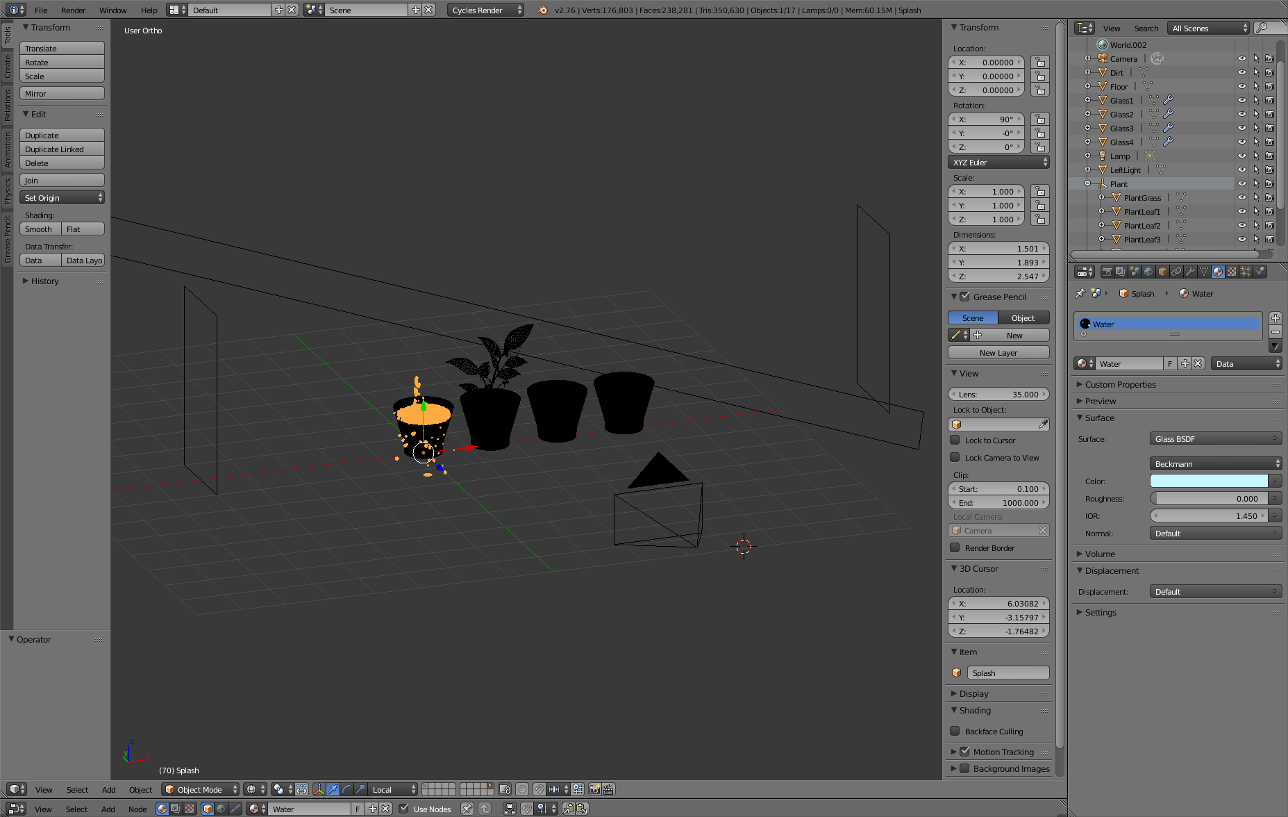
Blender Screen shot 1
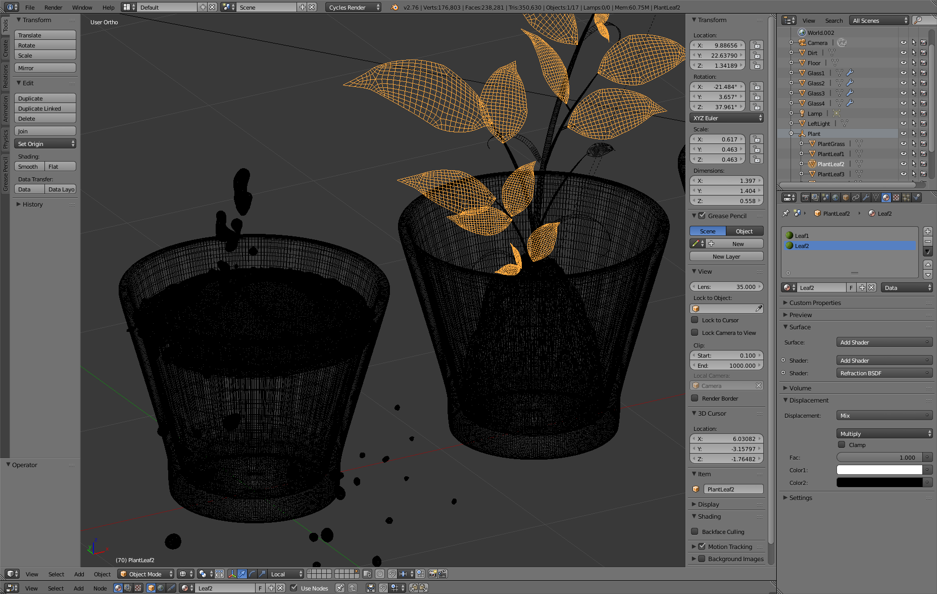
Blender Screen shot 2
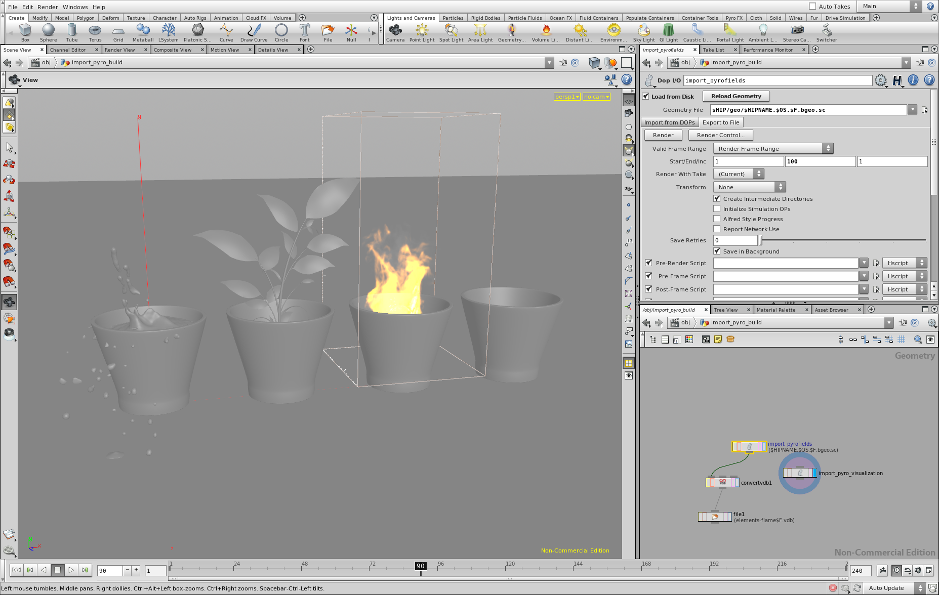
Houdini FX Screen shot 1
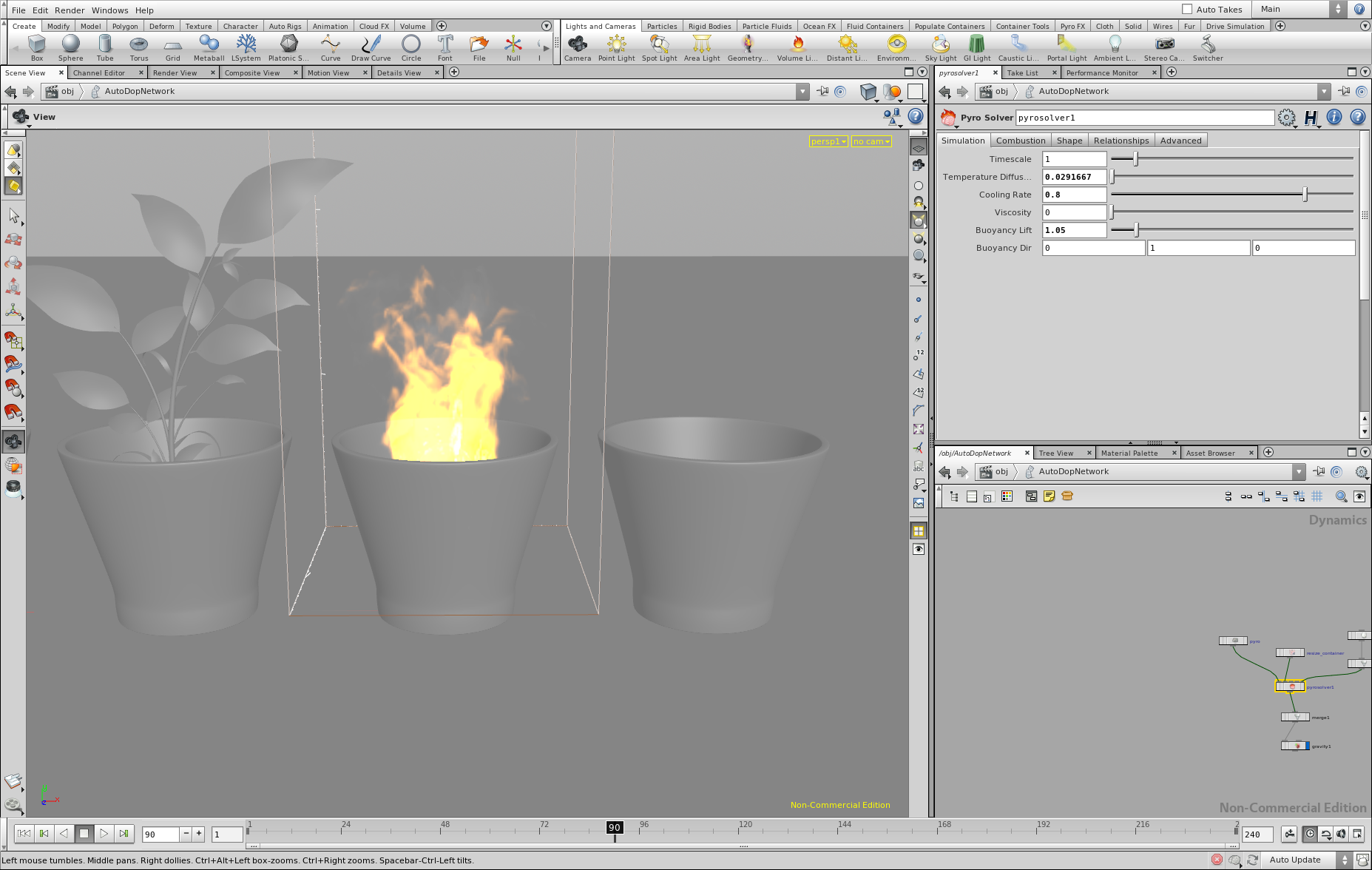
Houdini FX Screen shot 2
Final Image
The final image was rendered in 20 hours on an Intel Core-i7 at 1920x1080 resolution. There is a lot that could be optimized, but I was running out of time. Ironically, the adaptive sampler spent most of the samples on the dirt inside the second glass, which is the part of the image I dislike the most.
Final image
References
- [1] Physically Based Shading at Disney
- [2] Implementing Disney Principled BRDF in Arnold
- [3] Disney BRDF Viewer
- [4] A Realistic Camera Model for Computer Graphics
- [5] Monte Carlo Rendering with Natural Illumination
- [6] Microfacet Models for Refraction through Rough Surfaces
- [7] Generalization of Lambert’s Reflectance Model
- [8] Sobol Sampler by Leonhard Grünschloß
- [9] Production Volume Rendering
- [10] Multiple Importance Sampling for Emissive Effects
- [11] Importance Sampling Techniques for Path Tracing in Participating Media
- [12] Wikipedia - Thin Lens
- [13] A Hierarchical Automatic Stopping Condition for Monte Carlo Global Illumination
- [14] Robust Denoising using Feature and Color Information
- [15] Approximating Film with Tonemapping