Final Project Report
“That belongs in a museum”
Inspiration
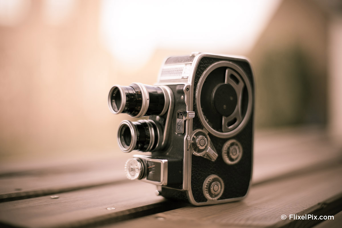
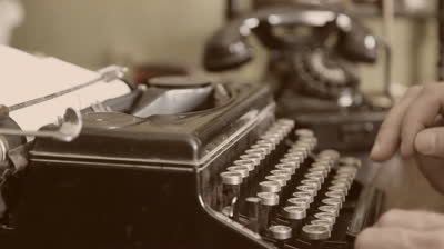
The goal for the final project is to create an image of an old camera, or an old typewriting machine (depending on what models will be available). A lot of effort will be put into creating believable materials, that have an old/dusty/used look. Also, the image should have a very photographic look, which is achieved by using physical camera model with a shallow depth of field. If render times permit, the space around the model could be filled with a inhomogeneous participating medium, to suggest a hint of dust in the air.
Overview
Due to lack of inspiration, I named my renderer skr (guess what it stands for). Apart from the math code provided in the course framework, the renderer has pretty much been written from scratch. The software design is inspired both from pbrt2 and from the very excellent Mitsuba renderer. I have also used Mitsuba to do correctness comparisons where applicable.
Thirdparty Libraries
The rendering framework builds upon the following thirdparty libraries:
- Qt 5.2 for the GUI
- libpic for loading/saving HDR images
- OpenEXR for loading/saving EXR images
- lodepng for loading/saving PNG images
- stb_image for loading JPEG images
- embree2 for efficient BVH acceleration structure
- pugixml for parsing/generating XML scene files
- serialize for serializing binary data
- tinydir for listing directories (cross-platform)
- tinyformat for typesafe printf-style string formatting in C++
- TinyObjLoader for loading Wavefront OBJ files
Simple Features
GUI
For improved usability of the renderer, especially with respect to the rendering competition, which would require quite a bit of tweaking, I decided to build a GUI to enable simple scene editing and parameter editing. The GUI is completely decoupleded from the rendering core, so it should be easy to build a standalone commandline based renderer at a later point. The GUI is built on top of the Qt 5.2 library and implements the following functionality:
- Loading, saving, merging scenes
- Importing Wavefront OBJ geometry
- OpenGL based preview with interactive camera placement
- Scene hierarchy view showing all the objects in the scene (Cameras, Lights, Objects, Materials etc.)
- Object inspector showing all parameters of a selected object for tweaking
- Render view with zooming/panning and interactive exposure and gamma controls
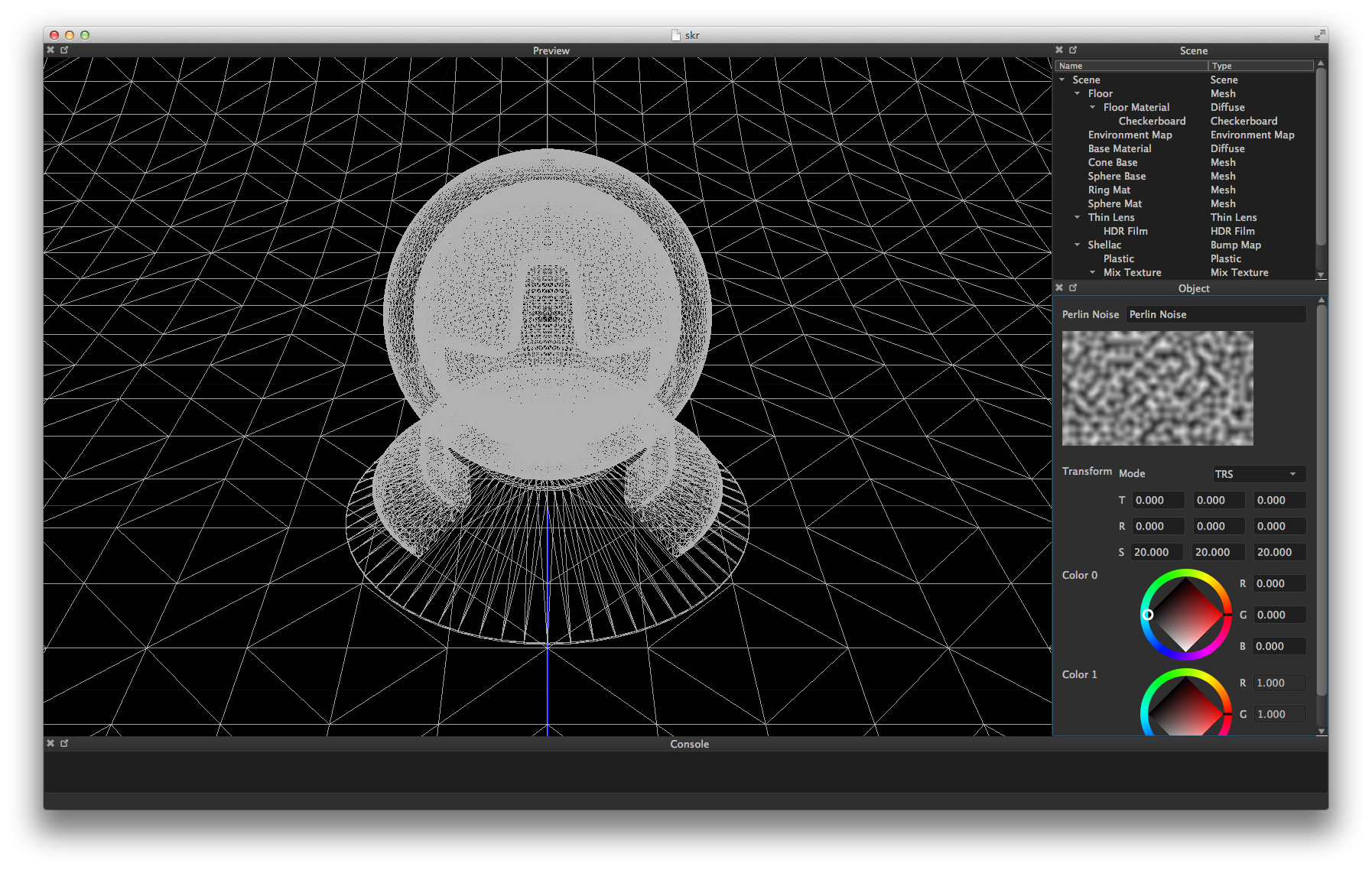
Image I/O
In order to support various image formats, the following libraries have been integrated into the framework:
- HDR (read/write) - libpic
- EXR (read/write) - OpenEXR
- PNG (read/write) - lodepng
- JPEG (read-only) - stb_image
Acceleration Structure
In the beginning, the framework used an adapted version of the BVH code from pbrt2. To improve performance at a later stage in the project, I switched to Intel's embree2 library, which is a highly optimized BVH implementation. This resulted in an overall speedup of over a factor 2x. During ray/scene intersections, two BVH instances are used, one to handle analytic primitive shapes such as spheres, planes etc., and a second one to handle triangle meshes. For simplicity and improved performance, all triangle meshes are transformed to world coordinates and put into the same BVH. The current implementation uses the pbrt2 adapted BVH for primitive shapes and the embree BVH for triangle meshes. For each ray/scene intersection (Scene::intersect), both BVHs are queried and the nearer hitpoint is returned. Due to the abstract interfaces Accel and TriangleAccel, it should be easy to extend the framework with additional acceleration structures.
Physical Camera
In order to create realistic renderings we need a realistic camera model. As a hobby photographer, I like to think in terms of sensor size, focal length and f-stops to control the camera. This is represented in the renderer by exposing a camera model with said properties. Using simple equations, we can then easily compute the required values used to generate primary rays in the renderer. First, we can calculate the field of view using the following equation:


Canon 5D with 50mm f/8
skr 50mm f/8
Canon 5D with 50mm f/4
skr 50mm f/4
Canon 5D with 50mm f/2
skr 50mm f/2
Canon 5D with 50mm f/1.4
skr 50mm f/1.4
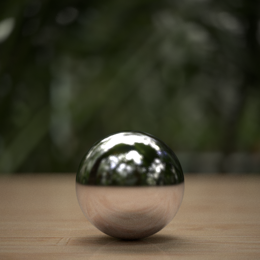
For artistic control, I have implemented a few additional features into the camera model. First, we can use a circular or rotated n-gon shape for aperture sampling. This allows controlling the appearance of the bokeh. The images above were rendered using a circular aperture, the images below are rendered with a 5 bladed aperture. Also, using an aperture bias parameter, samples taken in the aperture sampling routine can be shifted towards the edge or the center of the aperture. This is shown in the image below. Also, I have experimented with a simple trick to render the "cat's eyes" effect, by adding a virtual aperture between the the sensor and the front lens, in order to reject samples towards the edge of the lens. This results in the "cat's eyes" effect shown below. Note that at the same time, we also get vignetting, due to some of the light lost towards the edge of the lens.
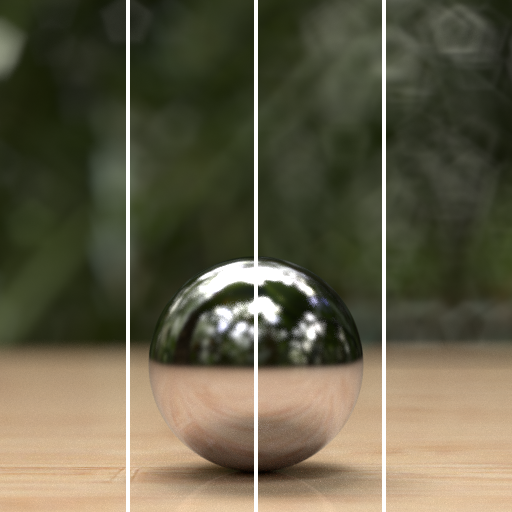
Aperture bias (0.0, 0.1, 0.2, 0.5 from left to right)
"Cat's eyes" effect
Creating camera rays is implemented in ThinLens::sampleRay. The aperture sampling is implemented in ThinLens::sampleAperture.
Mesh Lights
To allow for light sources of arbitrary shape, I have implemented diffuse area lights, which can sample from any of the implemented shapes. This also includes support for sampling from triangle meshes. The implementation builds upon the sampling interface provided by the Shape class, especially sampleDirect and pdfDirect, which implement sampling with respect to solid angle from a given reference point, and allow shapes to either use area based sampling together with domain transformation or directly sample with respect to solid angle. For mesh lights, we sample the mesh surface with respect to area and then use domain transformation. The area sampling first selects a triangle using the DiscretePdf1D class and then samples the choosen triangle uniformly.
For verification I have rendered a simple scene with a sphere light and compared it to a scene with a spherical mesh light. The comparison also shows the superiority of the sphere light sampling, resulting in much reduced variance compared to the mesh light. The difference image on the right clearly shows that lighting profiles are identical and the only difference is in the silhouette of the analytic sphere compared to the mesh sphere.
Left: Sphere light / Right: Mesh light (128 spp)
Difference between sphere light and mesh light (1024 spp)
Image Based Lighting
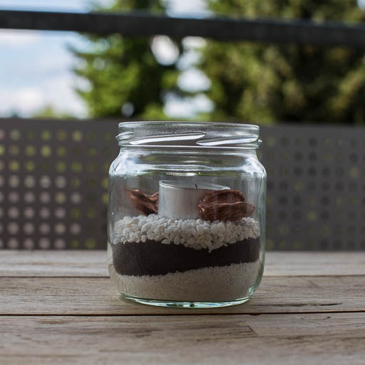
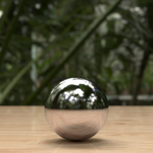
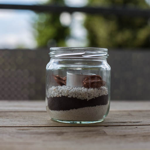
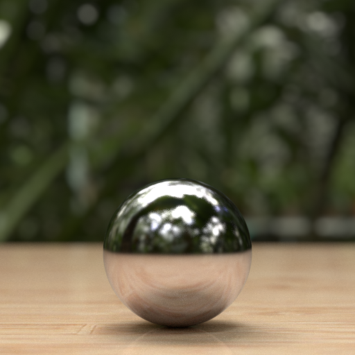
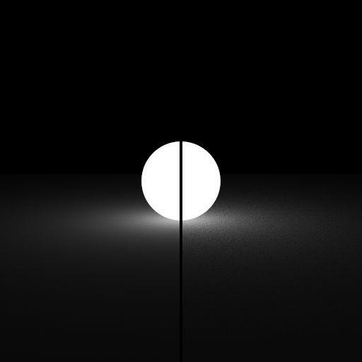
To allow for natural and realistic lighting, I have implemented lighting from HDR envrionment maps. In order to reduce variance, importance sampling as described in [1] was implemented. The following two images show the same scene rendered with and without importance sampling. The first showing the superiority of importance sampling by comparing visually, the second showing the difference between fully converged images, demonstrating correctness of the importance sampling. The third image shows a visualization of the importance sampling scheme.

Left: Without IS / Right: With IS (64 spp)

Difference between disabled/enabled IS (4096 spp)
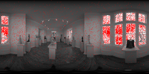
Visualization of the PDF generated from the luminance of the environment map and a set of importance sampled points
Medium Features
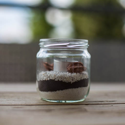
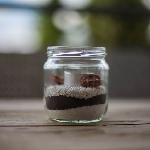
For my medium features, I mainly focused on rendering realistic materials, which would greatly help in creating the final image. This required the implementation of various BSDFs as well as a flexible texturing system. In order to test the BSDFs, I created a material test scene which I used to compare the results from skr with references from Mitsuba.
BSDFs
All BSDFs inherit from the common base class BSDF. As most BSDFs have multiple lobes (reflection, transmission etc.), they hold a list of components (lobes) and expose a lobe signature described using the EBSDFType enum. Each BSDF has to implement 3 basic methods:
BSDF::samplesamples an exitant direction, given an incident direction and a set of requested lobes. Returns the value of the BSDF divided by the PDF (for improved efficiency and numerical stability), pre-multiplied with the foreshortening term.BSDF::evalevaluates the BSDF given an incident/exitant direction, a set of lobes and a measure. Returns the value of the BSDF pre-multiplied with the foreshortening term.BSDF::pdfcomputes the PDF given an incident/extiant direction, a set of lobes and a measure.
BSDFQuery object as an argument, which holds, depending on the type of query, an incident direction, an exitant direction, and a set of requested lobes. When performing sampling, the sampled component is stored in the query object for later use. The measure argument specifies if the BSDF is evaluated with respect to solid angle or with respect to a discrete measure, used in lobes that describe a delta distribution.
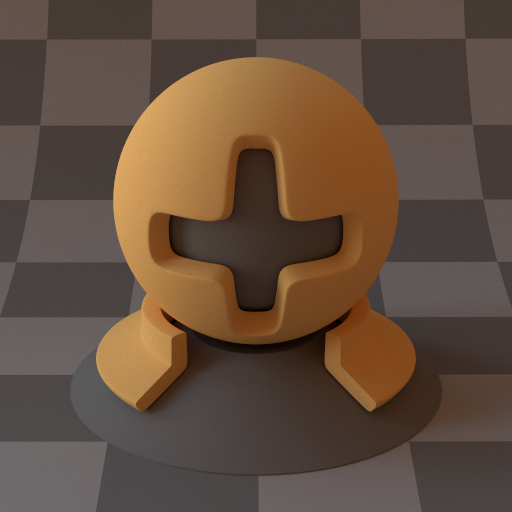
Diffuse
Implements the diffuse lambert BRDF using cosine-weighted sampling.
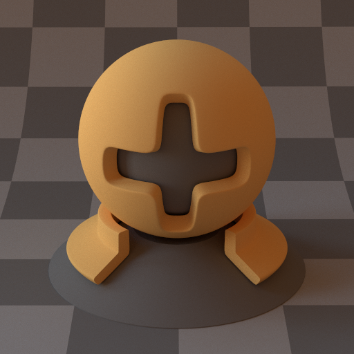
Diffuse BRDF rendered with skr

Diffuse BRDF rendered with Mitsuba
Dielectric
Implements a dielectric BSDF using the fresnel equations to model the interface between two dielectrics. The implementation uses russian roulette to decide between reflecting a ray and transmitting a ray, with a probability based on the fresnel reflectance computed in fresnelDielectricAuto.
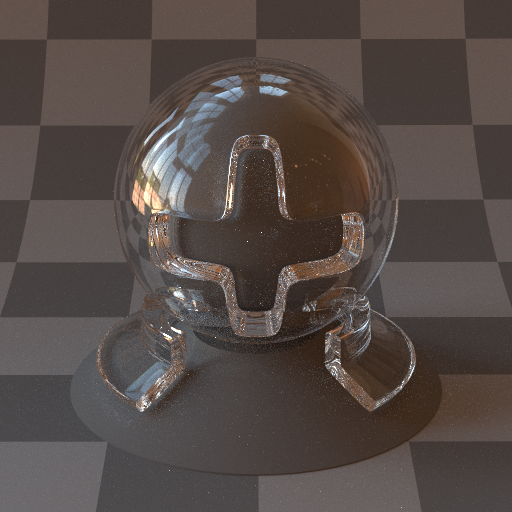
Dielectric BSDF rendered with skr

Dielectric BSDF rendered with Mitsuba
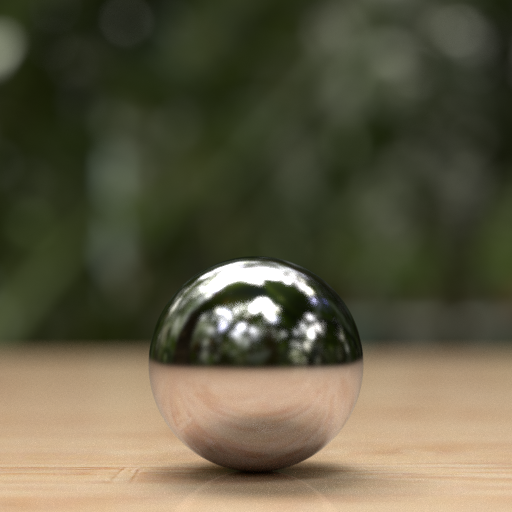
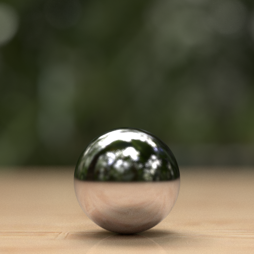
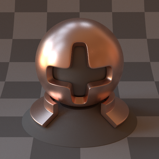
Conductor
Implements a conductor BRDF using the fresnel equations to model the interface between a dielectric and a conductor. The implementation uses the exact fresnel equations implemented in fresnelConductorExact, which are described in [4]. For physically plausible materials, the BSDF can be configured to use measured index of refraction data found in Mitsuba. The wavelength dependent eta and k values describing the index of refraction are convolved with the CIE curves to get RGB coefficients.
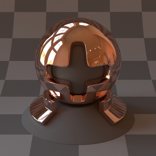
Conductor BRDF (copper) rendered with skr

Conductor BRDF (copper) rendered with Mitsuba
Phong
Implements the modified phong model. I didn't really use this BRDF for anything due to it's lack of realism.
Phong BRDF rendered with skr

Phong BRDF rendered with Mitsuba
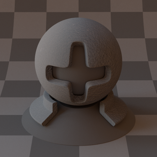
Rough Diffuse
Implements the Oren-Nayer BRDF as described in [2]. For simplicity, I only implemented the Qualitative Model as described in section 4.4 in the paper. For compatibility to Mitsuba, I also included the conversion factor to get a sigma for the Oren-Nayer model which behaves similarly to the roughness value in the Beckmann distribution (see below):

Rough Diffuse BRDF rendered with skr

Rough Diffuse BRDF rendered with Mitsuba
Microfacet BSDFs
In order to model rough dielectrics and conductors, I have implemented rough BSDFs as described in [3]. The paper gives a full overview for the implementation of microfacet BSDFs for dielectrics and conductors. As a first step, I have implemented the micro facet distributions that describe the statistical distribution of surface normals. The paper describes 3 distributions, namely Beckmann, GGX and Phong. All of them are described in section 5.2 of the paper and are implemented in the MicrofacetDistribution class. This class provides an interface to sample a normal, evaluate the distribution, compute the PDF of the micro normal and compute the shadowing term:
samplesamples a micro normal given a roughness valueevalevaluates the distribution given a roughness value and a micro normalpdfevaluates the PDF of the distribution given a roughness value and a micro normalGcomputes the shadowing term given a roughness value, an incident/exitant direction and a micro normal
Rough Dielectric
Implements a rough dielectric as described in equations 19, 20 and 21 in [3]. Uses the MicrofacetDistribution class to sample and evaluate the microfacet distribution. Analogous to the smooth dielectric BSDF, fresnelDielectricAuto is used to compute the fresnel reflectance coefficient as well as the refracted direction. To prevent extremely huge weights, I have also applied the lobe widening trick described in section 5.3.

Rough Dielectric BRDF rendered with skr
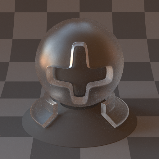
Rough Dielectric BRDF rendered with Mitsuba
Rough Conductor
Implements a rough conductor as described in equation 20 in [3]. Uses the MicrofacetDistribution class to sample and evaluate the microfacet distribution. Analogous to the smooth conductor BRDF, fresnelConductorExact is used to compute the fresnel reflectance coefficient.

Rough Conductor BRDF rendered with skr
Rough Conductor BRDF rendered with Mitsuba
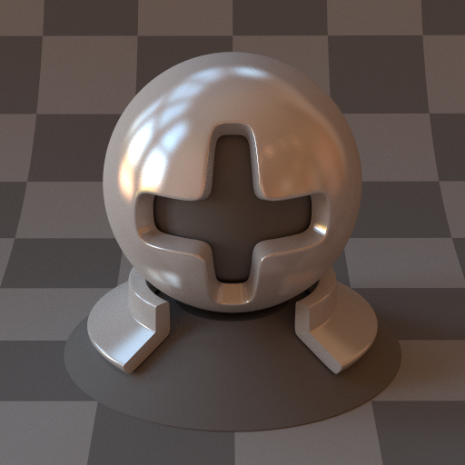
Plastic
Implements a plastic like material. A fresnel dielectric boundary is used to reflect light. The transmitted light is then assumed to diffusly reflect on the lambertian base layer and refract back through the dielectric boundary. Based on the implementation found in Mitsuba.
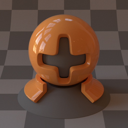
Plastic BRDF rendered with skr

Plastic BRDF rendered with Mitsuba
Diffuse Transmission
Due to input from Marios, I also implemented a diffuse transmission BTDF, which can be used to model the shading of a sheet of paper. It basically identical to the lambert diffuse BRDF, but mirrors the exitant direction to the other side of the shading frame.
Diffuse Transmission BTDF rendered with skr
Diffuse Transmission BTDF rendered with Mitsuba
Mixing
For more complex materials, it is useful to mix various BSDFs given an alpha texture. This is implemented in the mix BSDF.

Mixing between rough conductor and diffuse BRDF
Bump Mapping
For adding small perturbations into materials, I have implement a bump mapping BSDF, which basically just perturbs the shading frame and hands the sampling/evaluation to the nested BSDF. The perturbation of the frame is implemented as described in section 9.3 in the pbrt2 book. For simplicity and diminishing contribution, I left out the terms associated with the surface normal's derivative.
Diffuse BRDF with a perlin FBM bump map
Texturing
I have implemented a basic texturing system to allow for spatially varying properties on surfaces. All texture classes inherit from the Texture baseclass and implement the eval and evalMono methods. I have implemented the following texture classes:
Bitmaploading images from filesCheckerboard2Dprocedural 2D checkerboardConstantconstant colorGrid2Dprocedural 2D gridNormalDeviationprocedural texture evaluating normal deviation from a given directionMixTextureprocedural texture mixing two other textures with a third as a mix valuePerlin3Dsolid procedural Perlin NoiseFbm3Dsolid procedural Fractional Brownian Noise on top of Perlin Noise
Advanced Features
Volumetric Path Tracing
For my advanced feature, I decided to implement a basic version of volumetric path tracing. I started out with homogeneous and isotropic media and a naive path tracer.
Phase functions are implemented as subclasses of the PhaseFunction baseclass. They implement the usual sample, eval and pdf functions and use the PhaseFunctionQuery object for passing parameters and results (incident/exitant direction). The isotropic phase function is implemented in the Isotropic class.
Participating media are implemented as subclasses of the Medium baseclass. They implement two functions:
Medium::samplesamples a propagation distance on a given ray segment, and returnstrueif a propagation distance was sampled somewhere on the given ray segment,falseif there was no scatter event before reaching the end of the ray segment. Additionally, the sampled distance, transmittance to the scatter location and the PDF is stored in aMediumQueryobject. On success,pdfSuccessdenotes the probability of selecting the given propagation distance, on failure,pdfFailuredenotes the probability of choosing a point somewhere from the end of the ray segment to infinity.Medium::transmittancecomputes the transmittance along a given ray segment.
Homogeneous. To sample a propagation distance, it selects one of the RGB values of the extinction coefficient randomly and samples the distance exponentially. Then it uses MIS to compute a combined PDF based on all 3 color channels.
The naive volumetric path tracer is implemented in the class VolPathNaive. The basic procedure is the following:
- sample a propagation distance
- if scattering occured, adjust throughput and sample a new direction using the phase function
- if no scattering occured, adjust througput and sample a new direction using the BSDF at the surface
- if a light source is hit, terminate ray and add contribution
- use russian roulette to terminate recursion
As a first test scene, I set up a cornell box that is filled with a homogeneous isotropic medium. I used sigmaA = (0.01, 0.05, 0.09) and sigmaS = (0.5, 0.4, 0.3) for absorption and scattering coefficients. Then I compared the results from my renderer with results obtained from Mitsuba. As Mitsuba has two integrators based on volumetric path tracing (volpath and volpath_simple), I rendered the same scene with both integrators, and to my suprise found out, that the two integrators in Mitsuba did not match up. My results did match up with the volpath integrator in Mitsuba, and because the naive path tracer is quite simple in nature, I trust it to be correct and used my naive path tracer for comparsions in the tests to follow.
Left: skr / Right: Mitsuba volpath integrator (4096 spp)
Difference between Mitsuba volpath and volpath_simple
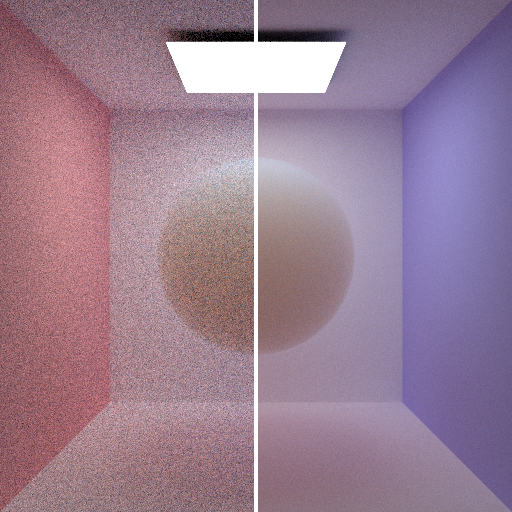
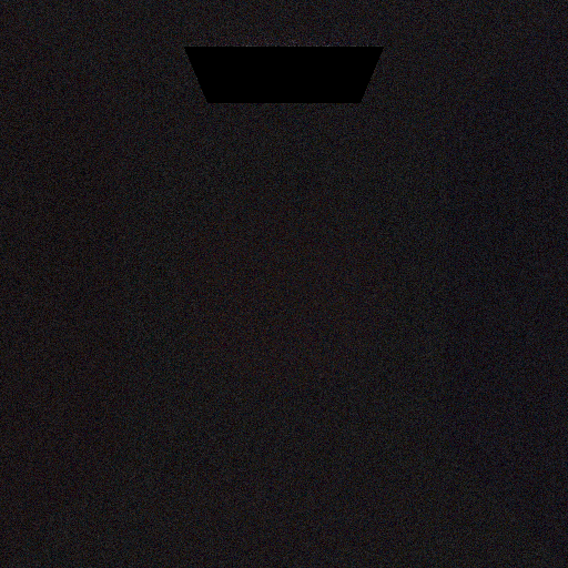
As a next step, I wanted to enclose my homogeneous media in arbitrary mesh boundaries. For this to work, I added a "forward" BSDF, which simply forwards incoming rays in a straight direction (implemented in the Forward class). As a test scene, I set up a cornell box with a sphere that contains a homogeneous medium and uses the forward BSDF on the boundary. I used sigmaA = (0.5, 0.7, 0.9) and sigmaS = (1.0, 2.0, 3.0) for absorption and scattering coefficients. This time, Mitsuba's integrators seemed to match up. The images below show the comparsion to Mitsuba. The difference image on the right is at +4 exposure values to show that there is only uniform noise due to sampling but no bias.
Left: skr / Right: Mitsuba volpath_simple integrator (4096 spp)
Difference between skr and Mitsuba with +4 EV
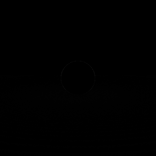
Multiple Importance Sampling
In order to reduce variance in the renderings with participating media, I have also written an improved version of the volumetric path tracer using importance sampling, combining the direct sampling of direct lighting with sampling of the phase function. This technique however, brings no real advantage as long as shadow rays are terminated at the first encounter of an intersection with geometry. This is why I had to extend the binary shadow rays with generalized shadow rays, which are allowed to pass through index-matched interfaces. To test this concept, I first implemented the generalized shadow rays in the basic path tracer that does not support participating media. This already has an advantage when rendering scenes that contain geometry which is only partially opaque. To enable partially opaque geometry, I first implemented the Masked BSDF, which allows an alpha map to specify the opacity. I then extended my path tracer with generalized shadow rays. The following shows a comparison rendering using a sphere that is only partially opaque. Note that when using binary shadow rays, we get a lot of variance, especially near the floor, where most shadow rays hit the geometry and prevent any contribution from direct lighting. Using generalized shadow rays however, we get the desired contribution from direct lighting, hence improve variance considerably. To show correctness, I rendered the same scene with binary and generalized shadow rays until convergence and took their difference.

Left: Binary shadow rays / Right: Generalized shadow rays (256 spp)

Difference between binary / generalized shadow rays (converged)
Next, I also implemented generalized shadow rays in the enhanced path tracer with support for participating media. This required shadow rays to not only account for opacity, but also account for transmittance along the ray. This technique, together with importance sampling, resulted in much reduced variance when rendering images with participating media. The following shows comparisons between the naive and the improved volumetric path tracer, using the test scenes for homogeneous media:
Left: Naive / Right: MIS (256 spp)
Difference between naive / MIS +4 EV (semi-converged)
Left: Naive / Right: MIS (256 spp)
Difference between naive / MIS +4 EV (semi-converged)
Heterogeneous Media
As a next step, I implemented heterogeneous media. In order to simplify sampling the propagation distance and evaluating the transmittance, I kept the heterogeneous medium monochromatic. The medium is configured with a spacially varying scalar extinction coefficient, further denoted as density. The scattering and absorption coefficients are then computed by a second spatially varying scalar value denoted as albedo. Using the following equations we can then derive the extinction, scattering and absorption coefficients:

Volume baseclass. The simplest being the Constant class, just returning a constant value. For spacially varying functions, VoxelGrid and decendent classes are used. The VoxelGrid just stores a 3-dimensional grid of scalar values. The descendents implement various functions to procedurally fill the grid with various functions.
To evaluate the transmittance in a heterogeneous medium, the query ray is intersected against the bounding box of the voxel grid, and then I use numerical integration using the trapezoidal rule to compute the density integral:

 is derived from the voxel grid and determines the number of steps
  to compute the integral. Using the density integral, transmittance is now easily computed using:
Heterogeneous::transmittance, the numerical density integration is implemented in Heterogeneous::integrateDensity.
To sample the propagation distance inside a heterogeneous, we can use the following equation:

 , and then uses numerical integration using the trapezoidal rule to compute the distance until the integrated density matches the left hand side. Sampling the propagation distance is implemented in
 Heterogeneous::sample and uses Heterogeneous::findDensity to find the distance travelled in the medium.
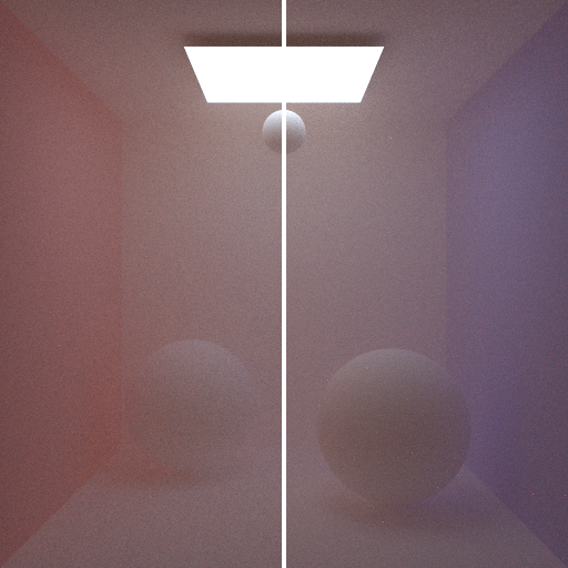
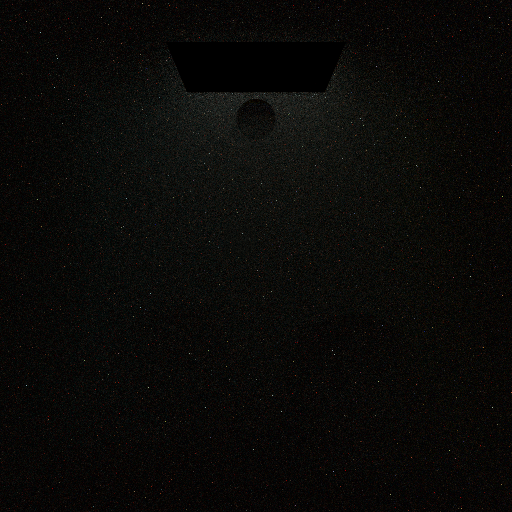
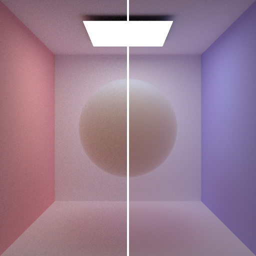
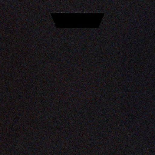
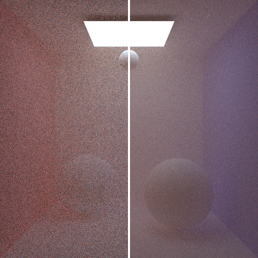
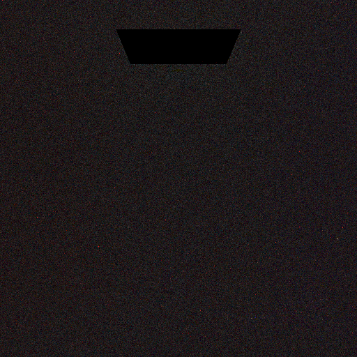
In order to validate the correctness of the implementation of heterogeneous media, I set up a test scene that contains a ball of fog. First, I rendered the ball using a sphere with a forward BSDF boundary that encloses a homogeneous medium. Second, I rendered the scene where the sphere is replaced with a heterogeneous medium with a density function defined by a 128x128x128 grid containing a solid sphere. The results are expected to be identical. The difference image on the right is at +4 exposure values, to show that there is only minor differences due to the finite resolution of the density function. Note that rendering with the heterogeneous medium is roughly 4x slower due to the overhead of raymarching.
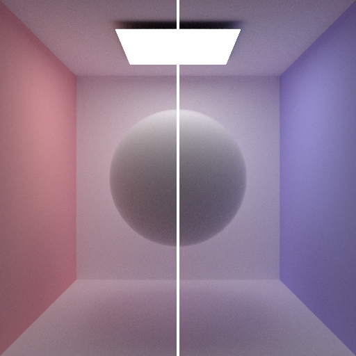
Left: Homogeneous medium / Right: Heterogeneous medium (512 spp)
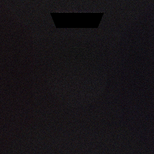
Difference between homogeneous / heterogeneous +4 EV (512 spp)
In order to render a more interesting image with a heterogeneous medium, I implemented a simple algorithm to compute a cloud like density voxel grid. The idea is derived from [6] and uses a simple distance function based around a sphere and a FBM to offset the boundary:

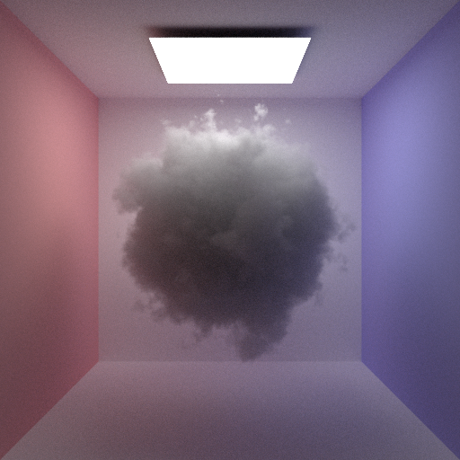
Pyroclustic density function (512 spp)
Additional Renderings
Some additional renderings done with volumetric path tracing.
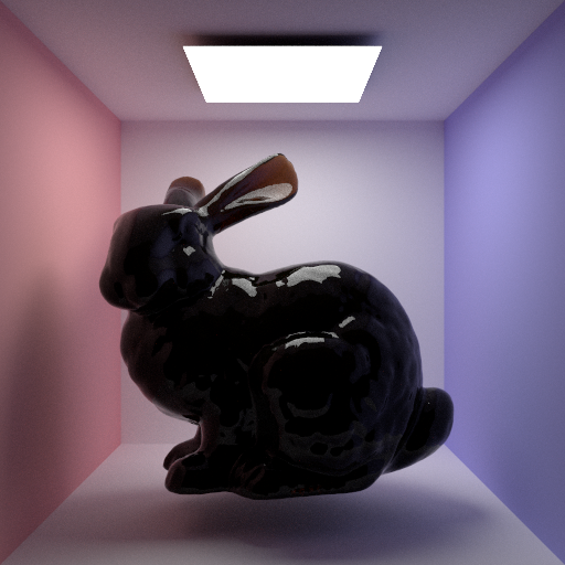
Coke Bunny
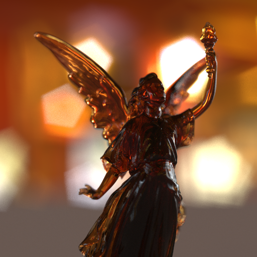
Beer Lucy
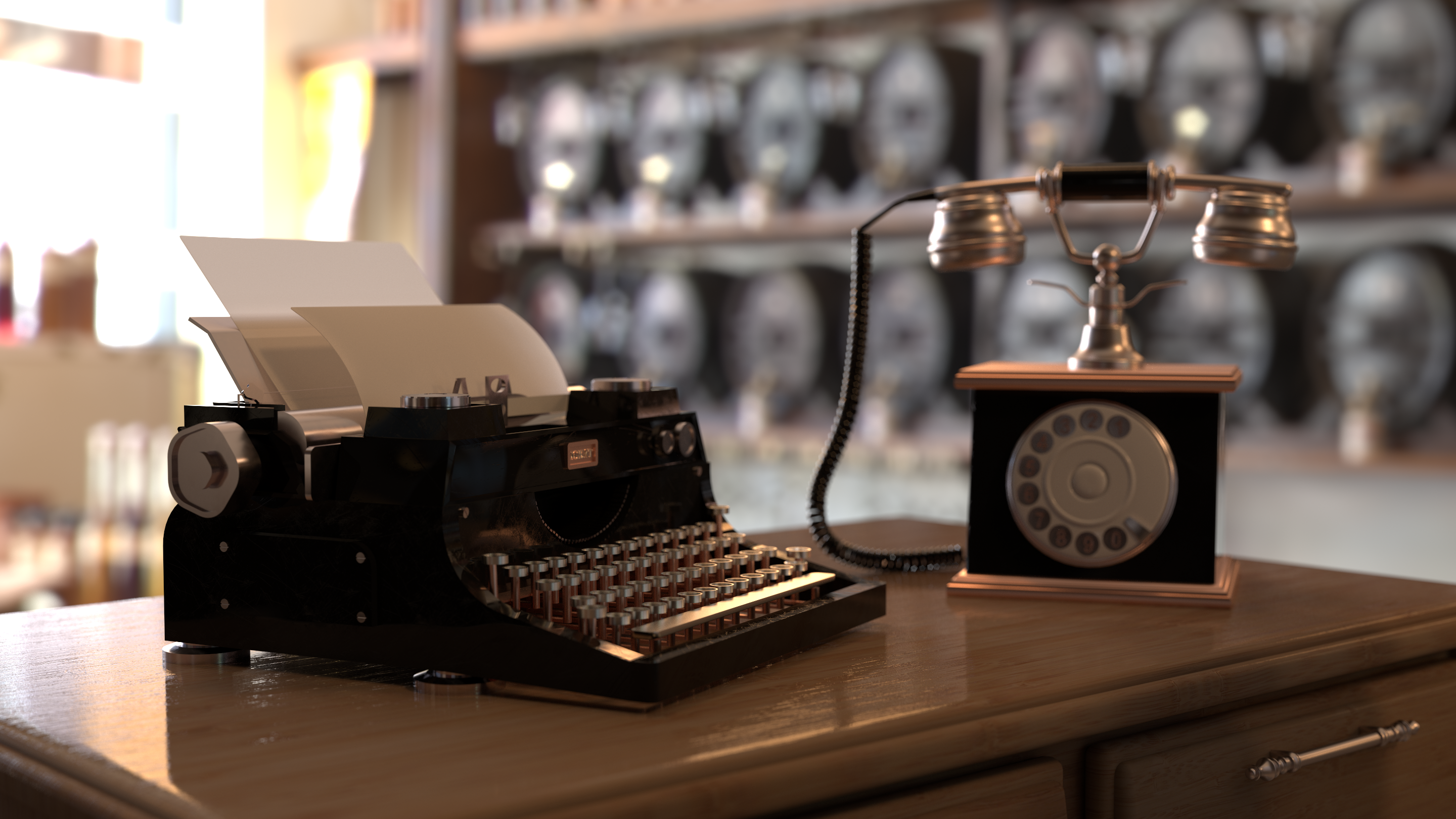
Final Image
For the final image, I only used a subset of the features implemented in the renderer. The idea to fill the scene with a heterogeneous medium turned out to be a bit over the top, as rendertimes with the current implementation would just go through the roof. Nevertheless, I was able to reach my initial goal of rendering an old typewriter and telephone. Quite a bit of time was needed to cleanup the models (which I got from the internet), create materials and textures, setup the scene and do the composition. To get a photorealistic look, lighting from an environment map as well as the camera model, that is configured with physically sound parameters, helped a lot. I also experimented with some other ideas, such as adding a thin layer of dust on the objects, using mixed materials based on the geometry normal, perturbed with noise functions, but it was difficult to get a good look. The first image shows the rendered image directly from my renderer. It has a resolution of 2880×1620 pixels and was rendered with 8k spp in roughly 6h.
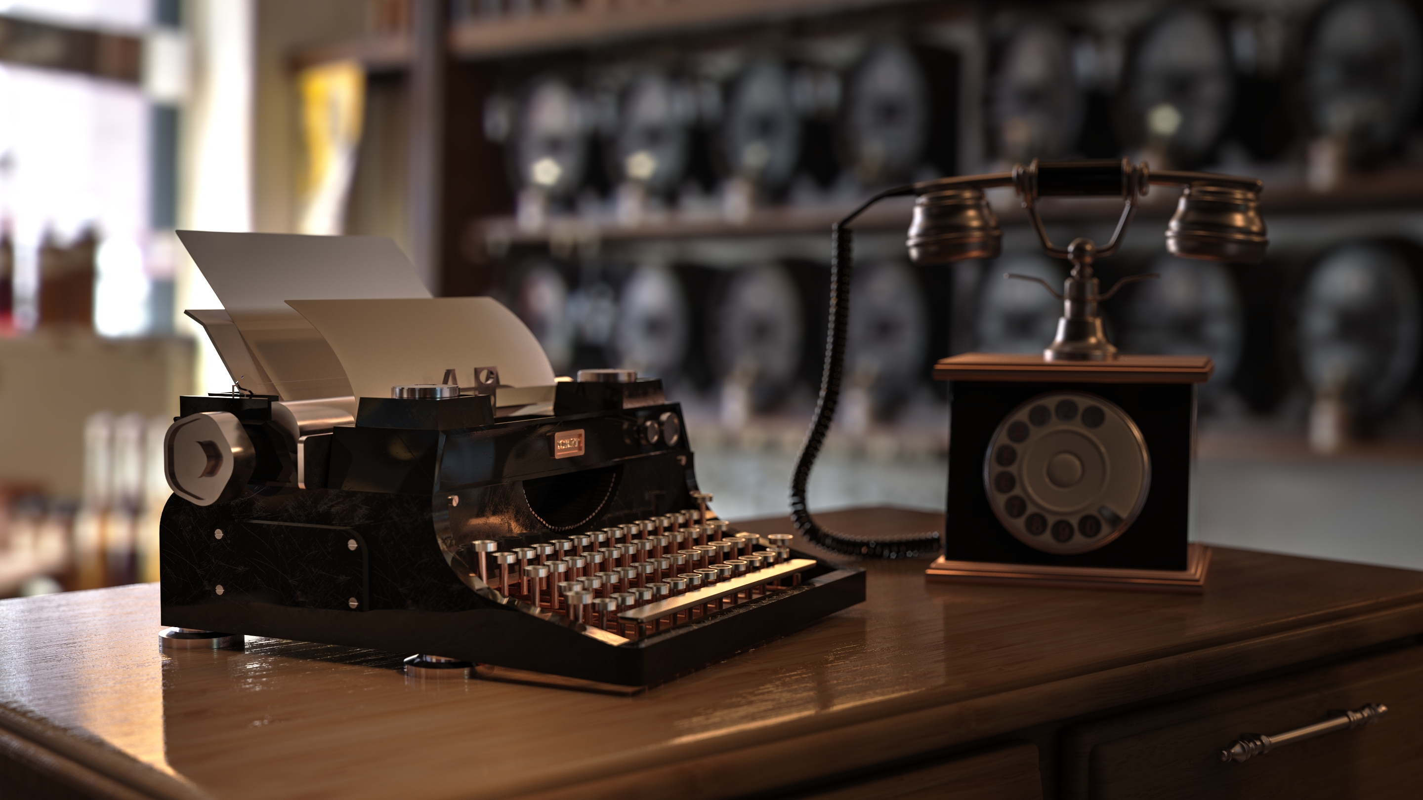
Due to having quite high dynamic range in the rendered image, I used Photomatix Pro to tonemap the image and bring back some of the details. I also removed a little bit of saturation and tuned the color temperature to my taste.
References
[1] Monte Carlo Rendering with Natural Illumination[2] Generalization of Lambert's Reflectance Model
[3] Microfacet Models for Refraction through Rough Surfaces
[4] Memo on Fresnel equations
[5] Unbiased Global Illumination with Participating Media
[6] Production Volume Rendering - Fundamentals